Where Should an Unattended Agent Think: The Cost-Quality Frontier of Reasoning-Budget Allocation Between Skill Selection and Execution
This post is for Korean cloud and AI engineers who run unattended agent loops or who answer for the thinking-token bill of such a loop. A production agent harness sends every incoming task to the skill/model router first and only then uses extended thinking in the execution stage. In current harnesses, most of the thinking budget is concentrated in the execution stage and the router is treated as a free classifier. Thinking tokens have become a priced, length-adjustable input. LLM re-ranking has made the router itself a per-request cost line item. Cheap latent-reasoning models keep pushing down the unit price of thinking tokens. With these three trends overlapping, the cost question for loops that run by the hour and the day has changed. It has moved from “should we think at all” to “where should we think”. The question this paper answers is how to allocate those tokens between the skill-selection stage and the task-execution stage. The goal is to maximize downstream task quality per dollar, given a fixed total thinking budget. It even prices how much extra routing accuracy (recall@5, top-1) and downstream quality a single router-stage thinking token buys over retrieval-only or no-thinking routing.
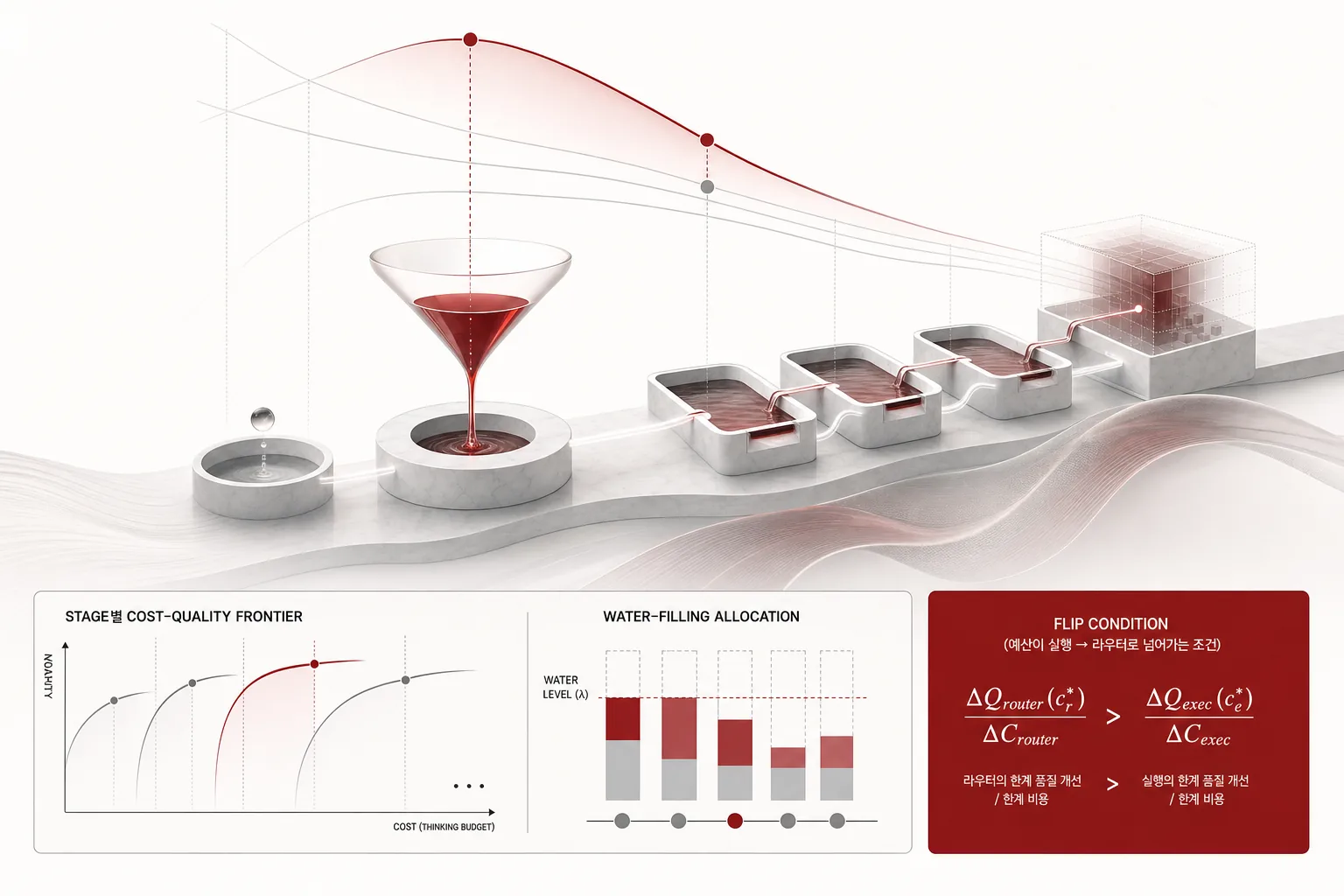 A visual metaphor for the article’s key idea.
In Plain Terms
When a patient arrives at a hospital, a triage nurse first decides which department to send them to. If that judgment is wrong, the patient goes to the wrong department and the examinations and surgery that follow are spent in full on thin air. Triage is cheaper and shorter than surgery, but every medical resource that comes after rides on that one judgment. Spend to make the triage judgment more accurate, or to make the surgery itself more precise? Is the shape of the allocation rule water-filling, where water fills the lower side first? At a hospital where triage is already almost always right, spending on surgery is the better move. At a hospital where triage misses a lot, spending on triage is the better move. This paper writes that “where” as a cost equation and gives the point at which budget moves from one stage to the other as an inequality.
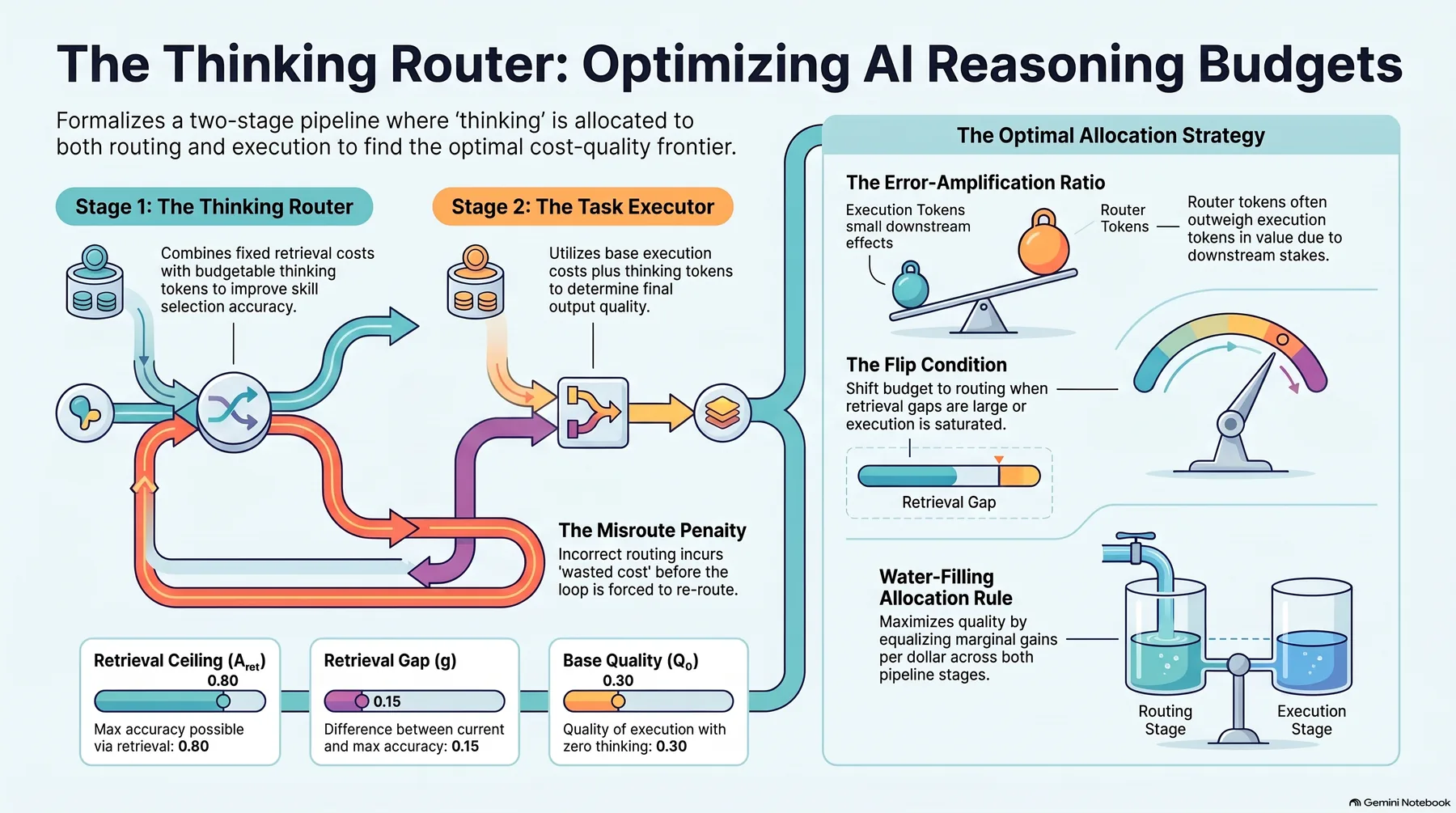 Infographic generated by NotebookLM from the sources.
The Router Treated as Free
The two-stage structure is simple. In Stage R (routing), a hybrid retriever (lexical + dense) builds the candidate pool at a fixed cost $b_R$. A thinking step for refining the selection spends $t_R$ at a token unit price $p_R$. Routing accuracy $A(t_R)$ is the probability that the gold skill is inside the top-k pool, and on our production route bench we take it as recall@k ($k{=}5$). In Stage E (execution), the selected skill runs at a base cost $b_E$ with an extended-thinking budget $t_E$ at a token unit price $p_E$. Execution quality $Q(t_E)$ is the probability that the task is completed correctly given the right skill.
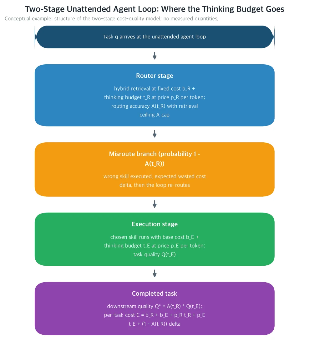 A conceptual diagram of the unattended agent loop as two stages. The next dollar is poured into the lower side until the remaining quality gain per dollar is equal across the two stages. Most current harnesses have the router doing retrieval only, with no thinking, and put all of the thinking into execution. In the language of water-filling, the water levels of the two stages are misaligned. The routing stage carries a fixed retrieval cost $b_R$ (lexical + dense retrieval) and a budgetable thinking cost $p_R t_R$, while the execution stage carries a base cost $b_E$ and a thinking cost $p_E t_E$. A misroute (probability $1-A(t_R)$) costs an expected waste of $\delta$ until the loop routes again. A conceptual illustration showing the structure of the two-stage cost-quality model. (Analytical model, not measured)
That router sits on the hot path of every turn. In our measurements, the embedding half of the hybrid skill router is not distributed offline but is looked up on every single request. The execution stage spends most of the tokens, but the router is a cost line item on every request as well.
Three trends change that picture. First, thinking tokens have become a priced, length-adjustable input. Thinking length tunes the cost-quality tradeoff of a single generation. Second, the router is no longer free. LLM re-ranking has made the selection step a per-request cost line item. Third, cheap latent-reasoning models are compressing the price of thinking tokens. So for a loop that runs by the hour and the day, where to think becomes a binding cost question.
Earlier work pinned down the retrieval cost of the router. The quantization study measured that the dense-embedding half is the first-order cost item and that its compression error decays through the fusion weight. The multi-skill gap study measured that in a 2,275-skill production registry the top-20 pool misses the gold skill of composite tasks 24.3% of the time. The binding constraint was coverage on the retrieval side, not the local composer’s ability. A local composer of $\le$14B produced 0 parseable chains out of 48. The repair loop study showed that the retriever’s cross-lingual vocabulary bridge is the co-binding constraint on step coverage. A hand-built oracle decomposition still left step coverage at 63.6%. In all three studies the router’s thinking budget was implicitly 0. The router either did not think, or if it did, the cost did not enter the accounting. This paper fills that gap.
The Cost Model: One Misroute Pays for the Whole Run
The expected cost per task is $C(t_R,t_E) = b_R + p_R\, t_R + b_E + p_E\, t_E + (1-A(t_R))\,\delta$. $\delta$ is the expected dollar cost of a misroute: the tokens spent executing the wrong skill plus the follow-on re-routing cost until the loop recovers or aborts. Prices are the list price for API arms and depreciation cost for self-hosted serving (e.g., an H200-class GPU). In the accounting, both enter as the same scalar.
Quality factors multiplicatively under the zero-credit misroute assumption. The assumption is that a misrouted task contributes nothing to a correct completion on the first attempt, and under it the downstream task quality is $Q^*(t_R,t_E) = A(t_R)\,Q(t_E)$.
For a total thinking budget $B$ (in dollars), the stage-level frontier is $F(B) = \max_{t_R,t_E \ge 0}\; A(t_R)\,Q(t_E) \quad \text{s.t.} \quad p_R t_R + p_E t_E \le B$. The frontier records the best downstream quality for each total thinking spend, and the argmax records the budget split that achieves it. There are four assumptions. A1 separability: $A$ depends only on $t_R$ and $Q$ only on $t_E$. A2 saturating response: both are differentiable, monotonically increasing, and strictly concave. The ceilings are $A^{\cap} < 1$ and $Q^{\infty} \le 1$. The former is a retrieval ceiling, where a skill the corpus does not describe will not surface no matter how much router thinking there is. Also $A(0)=A_{\mathrm{ret}}>0$ and $Q(0)=Q_0>0$. A3 stationarity: the task mix, the skill registry, and the description corpus are fixed over the measurement window. A4 price constancy: $p_R, p_E, b_R, b_E, \delta$ are constant over the same window.
The asymmetry shows up in the marginal values. The marginal quality of a router token is $\partial Q^/\partial t_R = A’(t_R)\,Q(t_E)$, and the marginal quality of an execution token is $\partial Q^/\partial t_E = A(t_R)\,Q’(t_E)$. The marginal cost of a router token is $p_R - \delta\,A’(t_R)$, and the marginal cost of an execution token is $p_E$. As routing gets more accurate, the expected misroute cost falls, which is why the router token carries a negative term in its marginal cost.
The Structure That Makes a Router Token Outweigh an Execution Token
This asymmetry is what the paper’s title points at. The quality revenue of a router thinking token, $A’(t_R)\,Q(t_E)$, is multiplied by the entire downstream execution quality. One unit of routing accuracy protects, or in the case of a misroute throws away in full, the entire downstream execution spend. The revenue of an execution token, $A(t_R)\,Q’(t_E)$, is multiplied only by the routing accuracy. It is a local improvement on an already-chosen path. On top of that, the router token carries the negative marginal-cost term $-\delta\,A’(t_R)$, because each increment of routing accuracy erases expected misroute cost.
The amplification ratio $\rho$ writes this contrast as a single number. $\rho = \dfrac{A’(t_R)\,Q(t_E)\,/\,(p_R-\delta A’(t_R))}{A(t_R)\,Q’(t_E)\,/\,p_E}$, and when $\rho > 1$ the next dollar of thinking buys more downstream quality at the router than in execution, while when $\rho < 1$ the reverse holds.
There are two structural consequences. Holding quality fixed, $\rho$ increases in $\delta$. Environments where misrouting is expensive, that is, environments with a long downstream pipeline, order-sensitive composite tasks, or external side effects, systematically favor router thinking. And the total quality gain obtainable from router thinking of any size is capped by the retrieval gap $g = A^{\cap}-A_{\mathrm{ret}}$. For every $t_R$, $A(t_R)Q(t_E) - A_{\mathrm{ret}}Q(t_E) \le g\,Q(t_E)$. Conversely, if $g > 0$ and the router’s response is non-degenerate, some positive allocation to the router is strictly optimal.
This gap has already been measured. In the 2,275-skill Korean-English production registry, the top-20 pool misses the gold skill of composite tasks 24.3% of the time. That means the retrieval gap, and with it the headroom for router thinking, is largest in exactly the regime where composite work matters most.
Water Fills the Lower Side First: the Water-Filling Allocation Rule
Under A1~A2, with the canonical saturating forms $A(t) = A_{\mathrm{ret}} + g\,(1-e^{-a t})$ and $Q(t) = Q_0 + (1-Q_0)(1-e^{-b t})$ and $\delta = 0$, the frontier is achieved at a unique pair $(t_R^, t_E^)$: the pair where the marginal log-quality per marginal dollar of the two stages are equal to the same water level $\lambda^$. $\lambda^$ is the unique solution of the strictly decreasing scalar equation $p_R\, t_R(\lambda) + p_E\, t_E(\lambda) = B$, and bisection solves it to any tolerance in finitely many steps.
Read as an operating rule, it is simple. Spend the next thinking dollar where the normalized marginal quality per dollar is highest, and stop when the water levels of the two stages are equal.
Three behaviors stand out. Because $A(0)=A_{\mathrm{ret}}$ already covers most tasks, the frontier has a kink at small $B$. Below a threshold budget the execution-only allocation is optimal ($t_R^*=0$), and the router receives its first budget once the flip condition is met. As $B$ grows, the marginal quality of each stage saturates and the split is re-allocated toward the stage farthest from its ceiling. Usually that means the relative share of router spend keeps growing until the retrieval ceiling binds. If $\delta > 0$, the effective marginal cost of router thinking is $p_R - \delta A’(t_R)$. If $\delta A’(t_R) \ge p_R$, router thinking becomes a marginal cost reduction, and the rule fills the router budget up to the latency or API ceiling.
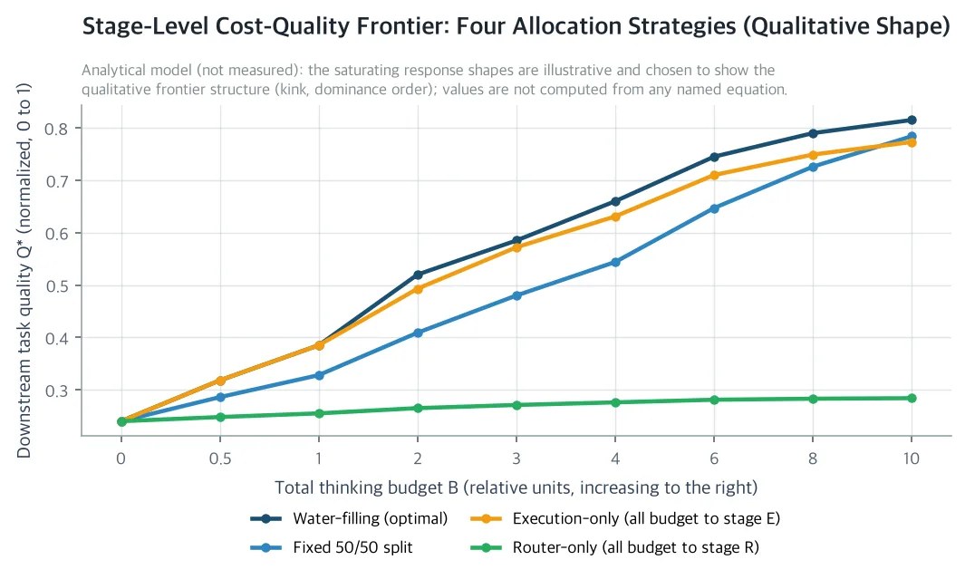 An illustrative model computation under assumptions A1~A2, not a measurement. Parameters: $A_{\mathrm{ret}}{=}0.80$, $g{=}0.15$, $a{=}0.01$, $Q_0{=}0.30$, $b{=}0.005$, $p_R{=}p_E{=}1$ (token-equivalent). The optimal water-filling allocation beats both fixed allocations at every budget level: below the small-budget kink it coincides with execution-only, and above it the edge over execution-only comes from filling the retrieval gap. The 50/50 split over-invests in the router before the router response saturates. (Analytical model, not measured)
The Flip Condition That Reverses the Direction of the Budget
When does the budget drop out of the router entirely? Letting $t_E^0$ be the execution-only optimum at budget $B$, the necessary and sufficient condition for the allocation that gives the router a zero budget to be optimal, at $\delta = 0$, is $\dfrac{A’(0)}{A(0)} \cdot \dfrac{Q(t_E^0)}{Q’(t_E^0)} \le \dfrac{p_R}{p_E}$. In the canonical forms $A’(0)/A(0) = a\,g/A_{\mathrm{ret}}$ and $Q(t)/Q’(t) = \dfrac{e^{bt}-(1-Q_0)}{b\,(1-Q_0)}$, so the condition becomes $\dfrac{a\,g}{A_{\mathrm{ret}}} \cdot \dfrac{e^{b t_E^0}-(1-Q_0)}{b\,(1-Q_0)} \le \dfrac{p_R}{p_E}$. With $\delta > 0$ the flip is delayed and the condition changes to $\dfrac{A’(0)\,Q(t_E^0)}{p_R-\delta A’(0)} \le \dfrac{A(0)\,Q’(t_E^0)}{p_E}$.
The flip condition is the paper’s headline rule. Router thinking is worth it when one of four things holds. When the retrieval coverage gap $g$ is large. When the router’s response speed $a$ is high, that is, thinking converts well into recall. When the execution stage runs deep on its saturation curve, where $Q/Q’$ is large and execution tokens are about to stop paying. When router tokens are relatively cheaper than execution tokens, the regime created by a cheap latent-reasoning model with a small $p_R/p_E$.
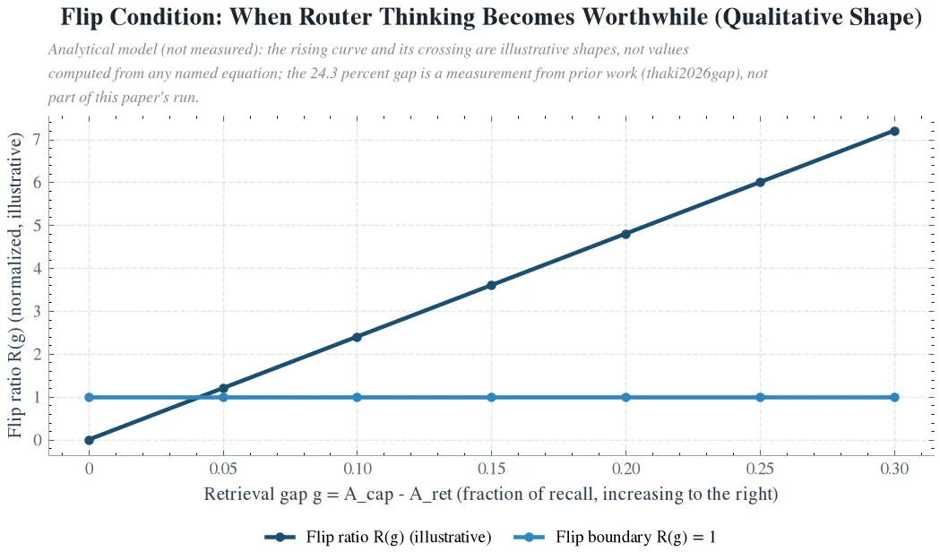 An illustrative model computation, not a measurement. With parameters $a{=}0.01$, $A_{\mathrm{ret}}{=}0.80$, $b{=}0.005$, $t_E^0{=}400$, $p_R{=}p_E{=}1$, $R(g)=23.9\,g$, so the router should receive a positive thinking budget once the retrieval gap passes $g\approx0.042$. The 24.3% top-20 coverage gap of the 2,275-skill production registry is a measurement from an earlier study, not a run of this paper. That value sits deep inside the region where thinking is worth it for the router. (Analytical model, not measured)
Retriever Compression and the Thinking Budget Do Not Substitute for Each Other
The earlier quantization result acted on $b_R$, not on $t_R$. INT8 quantization of dense embeddings lowers retrieval compute, and its accuracy error reaches the fused score only through the dense term, damped linearly by the fusion weight. To first order it is of size $w\,\epsilon$. The lever in this paper acts on $t_R$. Near $t_R = 0$, the thinking gain $A(t_R) - A(0)$ is of size $a\,t_R$. The two levers act on first-order distinct terms of the same frontier. $b_R$ compression moves the cost intercept with quality roughly unchanged, and a $t_R$ budget raises quality with the base cost roughly unchanged. The interaction is second order in $(\epsilon, t_R)$.
The practical consequence is that the two investments are not substitutes. A team that quantizes the retriever and spends the saved dollars on execution thinking has left the router-stage lever on the table. The frontier-optimal move is to re-solve the water-filling equation every time one lever is pulled.
The 5×3 Protocol for Measuring the Frontier on a Production Bench
The procedure for a router team to estimate the stage-level frontier on production infrastructure. Every quantity is defined to be auditable. Every arm reports stage-level token counts and per-task dollars.
There are five router arms. R0 retrieval-only: lexical + dense hybrid score, no LLM call in the selection decision. R1 zero-thinking re-rank: a compact LLM makes one fast forward pass over the top-20 pool with extended thinking off. R2: extended thinking at a small fixed budget $b_{\mathrm{low}}$. R3: $b_{\mathrm{med}} = 4\,b_{\mathrm{low}}$. R4: $b_{\mathrm{high}} = 16\,b_{\mathrm{low}}$. There are three execution arms. E0: no extended thinking. E1: $e_{\mathrm{low}}$. E2: $e_{\mathrm{high}} = 8\,e_{\mathrm{low}}$. A full factorial 5×3, 15 cells. Budgets are set in absolute tokens and renormalized when the underlying model generation changes, and the geometric spacing probes the shape of the saturating response (A2) without wasting spend.
The full factorial runs on a fixed task pool drawn from the production route bench. There are two strata. Single-skill versus composite tasks, with composites scored order-sensitively per the chain-benchmark convention. Query language, whether cross-lingual tasks sit where the retrieval gap is largest. Each cell receives the same tasks in the same order. A deterministic seed attributes differences across arms to budget rather than to task variation.
The measured metrics go by stage. Router stage: recall@1, recall@5, top-1 exact match, chain-level hit on composite tasks (all gold skills of the gold chain present in order). Thinking-token spend, router-stage dollars. Execution stage: task success (function-calling accuracy + final-state check), thinking-token spend, execution-stage dollars including tool-call and context costs. Loop level: per-task dollars (reporting list price and self-hosted depreciation separately), the expected misroute penalty $\hat{\delta}$ estimated from retry trajectories, downstream quality $Q^*$, quality per dollar, and the frontier point $(B, F(B))$ with its argmax split.
The estimation is isotonic regression. Fit the stage responses $\hat{A}(t_R)$, $\hat{Q}(t_E)$ over the arm budgets, assuming monotonicity but not shape. Read the frontier from the water-filling equation using the fitted responses, and put a 95% bootstrap confidence interval on each frontier point and each argmax split. The resampling is over tasks within strata. There are three guardrails. Saturation check: if $b_{\mathrm{high}}$ shows no significant recall gain over $b_{\mathrm{med}}$, the retrieval ceiling is near and the gap bound is in force. Flip check: re-evaluate the flip condition whenever the description corpus or the registry changes, because $g$ moves. Cost-drift check: drift of $p_R/p_E$ across model generations, because the flip condition is price-sensitive. The protocol re-runs periodically on a fixed bench slice. If any frontier point falls outside its confidence interval, that triggers a reallocation review rather than being left as a silent default.
Latency and Sequence Routing: Where the Frontier Meets Next
The answer the theory gives is conditional. Router thinking is worth it when the retrieval gap is large, misrouting is expensive, execution is saturated, and router tokens are cheap. If retrieval is saturated and execution still has headroom, router thinking is waste. That is why the frontier has to be measured per harness. The same model family sits on one side of the flip condition on a saturated single-skill registry and on the other side on a 2,275-skill bilingual registry.
Because the router runs every turn, its thinking budget is also a latency budget. A hard per-turn latency cap $L_{\max}$ cuts the feasible set to $t_R \le L_{\max}/r_R$ ($r_R$: router tokens per second). The water-filling rule applies to the cut set unchanged, and only $F(B)$ falls. Decision caching, reusing routing decisions for task families seen before, is a free first-order approximation worth measuring as a separate arm.
The flip analysis is about single-step selection. A composite task’s output is an ordered skill chain, and it grows the router’s decision. Since $\delta$ grows with chain length and order-sensitivity, moving the routing response $A$ can also become expensive. The router has to think at the sequence level rather than at the individual item level. The framework extends as-is by replacing $A$ with the chain-level hit rate. The paper expects the effect of misroute stakes raising the router’s value to be strongest exactly there.
So What Should You Change
First, a per-stage budget tuning rule is needed. That is a rule to match the normalized marginal quality per dollar across stages, and re-measure on the route bench and the function-calling harness. It also leaves the answer to whether the skill-selection stage is a cost-quality lever in our agent stack.
Second, treat retriever compression and router thinking as separate levers. Spending the dollars saved by quantizing the retriever on execution thinking alone leaves the router-stage lever on the table. The frontier-optimal move is to re-solve the water-filling equation every time one lever is pulled, and keep the optimal allocation.
Third, measure the frontier again on a fixed bench slice, on a recurring schedule. If a frontier point falls outside its confidence interval, trigger a reallocation review rather than leaving it as a silent default. Re-check the flip condition whenever the description corpus or the registry changes. The reason splitting the thinking budget by stage is an accessibility lever that lowers the bill for teams running unattended loops is here: when the token bill and the GPU energy per task both fall, autonomous workflow automation becomes affordable for teams that cannot carry the frontier-model bill per turn.
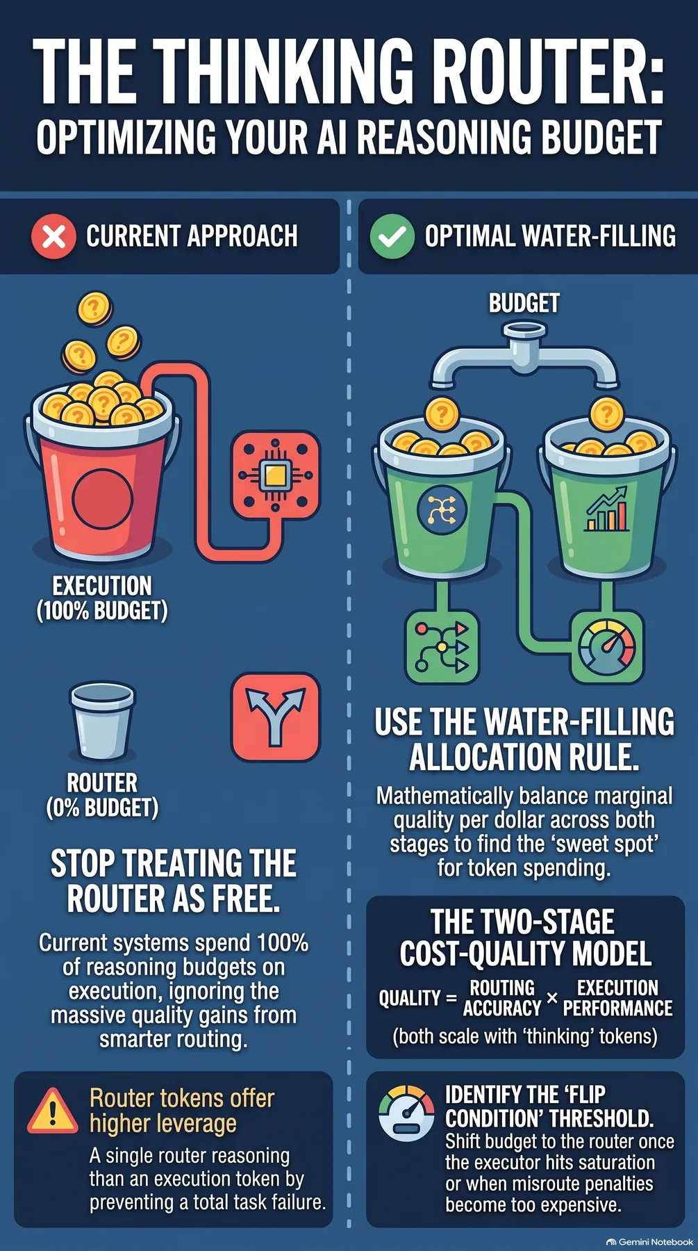 Infographic generated by NotebookLM from the sources.
What Cannot Be Trusted
This is an analytical paper. It sets up the allocation theory and the measurement design, and the frontier numbers here are illustrative model computations under A1~A2, not measurements. The only number that enters this post as a measurement is the 24.3% top-20 miss on the 2,275-skill registry from the previous post. Even that is a measurement from an earlier composite-task study, not a run of this paper.
A1 (separability) breaks when router thinking changes the task representation the executor sees, the case where the router emits a plan instead of a skill, in which case the analysis over-attributes execution quality to execution thinking. A3 (stationarity) is violated by a description repair that swaps the description corpus overnight, and the protocol’s flip check is the mitigation. The zero-credit misroute assumption (a misrouted task scores zero on the first attempt) is conservative for harnesses with robust retry. A positive-credit variant only lowers $\delta$ and delays the flip. In the water-filling and flip results, the canonical exponential form is for tractability, and the qualitative claims (a single water level, a monotone flip condition) hold for any saturating response under A2. The protocol itself is the check: re-measure periodically on a fixed bench slice, and treat a frontier point’s escape from its confidence interval as a trigger for a reallocation review.
The paper’s detail page is here: The Thinking Router: Measuring the Cost-Quality Frontier of Reasoning-Budget Allocation Between Skill Selection and Task Execution in Unattended Agent Loops
All three figures in this post are outputs of an analytical model, not measurements. The only number that enters as a measurement is the 24.3% top-20 miss on the 2,275-skill registry from the previous post.