Running a Coding Agent Fleet Costs $47K a Month at List Price. On Our Own GPU, $3,960.

If you’re running coding agents on a commercial API and the bill keeps growing, this is where to look first. Here’s the conclusion up front.

57 unattended agents spend a month’s worth of tokens that, converted to list price, comes to $46,911. Running the same work on a single B200 costs $3,960. That’s 12x. On the heaviest usage day, it’s $62,343 versus $3,960, a 16x gap.

And 90% of that bill wasn’t output tokens. It was cache reads. That’s also why the total barely moves whether you price it against Claude Code or Codex: the two vendors differ by only 1.7%. Both price cache reads at one-tenth of input, and that line item dominates the total. Self-hosting has no such line item at all.

The biggest single lever wasn’t switching models, either. It was two lines of serving configuration.

What a month costs

Here’s the summary table first: the same fleet’s token usage, repriced against each vendor’s list price.

Where it runs	Monthly cost (average)	Monthly cost (peak day)	Multiple
Codex (GPT-5.6 Sol)	$47,705	$63,375	12.0x
Claude Code (Opus 5)	$46,911	$62,343	11.8x
Claude Code (Sonnet 5)	$28,147	$37,406	7.1x
Codex (GPT-5.6 Terra)	$19,082	$25,350	4.8x
Self-hosted (1x B200)	$3,960	$3,960	baseline

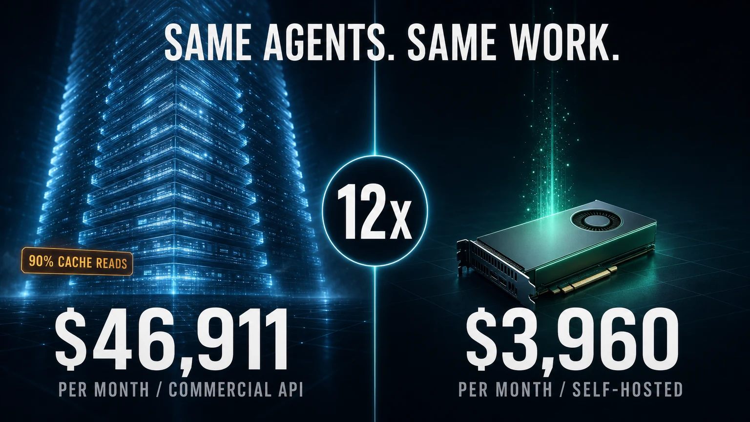The same agents do the same work. The only thing that changes is where it runs.

The top two tiers land within 1.7% of each other. Switching models doesn’t move you an order of magnitude. Dropping a tier gets you to about half, which is still nowhere near 12x.

It also matters that the self-hosted column is flat regardless of usage, since GPUs are rented by the hour, not by the token. The rest of this post is about why those two columns split apart the way they do.

We opened up the bill first

We run 57 unattended runners. A nightly paper factory, a news digest, a blog-evolution pipeline, sales briefs, self-QA: things that wake up at a fixed time, do their work, and go back to sleep. With no one watching, usage quietly piles up.

We converted this fleet’s daily token usage to commercial API list price. Here’s the last three days.

Date	Input	Output	Cache reads	List price
2026-08-13	2.63M	5.39M	2.34B	$1,429.90
2026-08-18	2.90M	3.60M	1.80B	$1,151.63
2026-08-19	3.22M	6.88M	3.78B	$2,202.12

What caught our eye first wasn’t the total. It was the cache-read column. Fresh input is 3.22M, and cache reads are 3.78B, over a thousand times larger.

Every turn, an agent resends its entire system prompt, skill definitions, and conversation history so far. Most of that hasn’t changed a single character since the previous turn, so it gets served from cache. Cache reads are priced at one-tenth of input, which looks cheap, but at a thousand-to-one volume, that line wins on total.

Breaking down 2026-08-19 by line item at Opus list price:

Item	Amount	Share
Cache reads	$1,890.00	90.9%
Output	$172.00	8.3%
Input	$16.10	0.8%

Hunting for a cheaper model to cut token unit price is fixing the 8%. The other 90% is somewhere else entirely.

On self-hosted, cache reads aren’t a billing axis at all

Commercial APIs sell tokens. Self-hosting buys GPU time. That difference becomes extreme exactly at the cache-read line.

vLLM’s prefix caching reuses KV that’s already been computed. Tokens that hit the cache skip prefill entirely. Attention still reads that KV during decode, but that cost is already folded into decode throughput: it isn’t a separate line item. The same 3.78B tokens are a $1,890 billing line on one side and don’t exist as a line at all on the other.

So self-hosted cost comes down to the two axes where compute actually happens: prefill and decode. Dividing our 2026-08-19 usage by measured throughput:

6.88M decode tokens divided by 4,150.7 tok/s comes to 0.46 GPU-hours. 3.22M prefill tokens comes to 0.16 GPU-hours. Combined, 0.62 GPU-hours for the day, 2.6% of one B200’s 24-hour day.

GPUs aren’t rented by the second, of course. Keeping one card on all day at $5.50/hour costs $132. Against that day’s list-price equivalent, that’s a 16x gap, and it’s where the $47K vs $3,960 monthly figures in the table above come from.

The remaining headroom is large, too. If we’re only using 2.6% of one card, we could grow the fleet more than thirtyfold and it would still run on that same card. The more agents you add, the lower the per-card unit cost drops.

Three levers, and the size order isn’t what you’d expect

We split the savings into three pieces and measured each one’s contribution.

flowchart LR
  A["Platform default<br/>231.6 tok/s<br/>$6.60 / 1M output"] -->|"Serving config<br/>17.9x"| B["Tuned<br/>4,150.7 tok/s<br/>$0.368"]
  B -->|"Quantization<br/>1.68x"| C["NVFP4 + FP8 attention<br/>size down 59%"]
  C -->|"8B distillation<br/>1.59x estimated"| D["Worker-only 8B<br/>2.0s latency"]
  style A fill:#7f1d1d,color:#fff
  style B fill:#1e3a5f,color:#fff
  style C fill:#14532d,color:#fff
  style D fill:#3f2d56,color:#fff

First, serving config: 17.9x

The biggest lever had nothing to do with the model. Same checkpoint, same GPU, same engine, and we changed two environment variables so saturated throughput went from 231.6 tok/s to 4,150.7 tok/s.

The culprits were TORCH_COMPILE_DISABLE=1, baked into the serving pod by the platform, and the chart default --max-num-seqs 32. The first left the engine running uncompiled, which put single-stream latency at 34.65 seconds. The second capped concurrent sequences at 32, fixing the throughput ceiling. The cost was 79 extra seconds of startup time.

$6.60 per million output tokens becomes $0.368. We didn’t change a single line of code.

Second, quantization: 1.68x

We quantized Qwen3.8-27B ourselves. A build with MLP in NVFP4 and attention/KV in FP8 goes from 2,141.4 tok/s to 3,586.3 tok/s at concurrency 128, versus bf16. Size dropped from 51.77 GiB to 21.34 GiB, a 59% reduction.

Quality held up on MMMU across 232 questions: McNemar test p-values ranged from 0.344 to 1.000. That means we couldn’t detect a loss, not that there is no loss, but at least in this sample, nothing separated the two.

When size drops by more than half, more sequences fit on the same card, and that feeds straight back into throughput. Quantization’s value is half speed, half density.

Third, the distilled 8B is less cheap than you’d think, but faster

We distilled an 8B model from the 27B’s execution traces. Parameters are 3.4x smaller. But the throughput gain is only 1.6x.

The reason is interesting. Qwen3.8-27B has 16 layers, so its per-token KV cache is unusually small; Qwen3-8B has 36 layers, so its KV cache is actually larger. Even with smaller weights, trying to grow the batch runs into KV claiming the space first. Estimating cost from parameter count alone is off by more than a factor of two.

Latency is where the difference is unambiguous, though. Across 15 bounded worker tasks, 8B’s median is 2.0 seconds against 27B’s 7.5 seconds. Both finish 15/15; format compliance is 13/15 for 8B and 15/15 for 27B.

Distillation itself was nearly free. 770 rows of training data, 14 minutes on a B200, which prices out to $1.28 at rental rates. Held-out spec compliance rose 26.5 points.

So how much does mixing them actually save

We opened a trace of an orchestrator handing sub-tasks to an 8B worker in production. The parent 27B made 13 LLM calls totaling 13,125 output tokens; the 8B worker made 8 calls totaling 917 tokens.

Worker output is only 6.5% of the total. Dropping that 6.5% to 8B saves 2.4% of cost. Honestly, that’s marginal from a cost standpoint.

The reason to use 8B isn’t cost. It’s that more sub-tasks finish in parallel in the same window, and the orchestrator spends less time waiting. Savings are a side effect. Sell this as a cost-savings project and the numbers won’t back you up.

The next step is letting 8B run the orchestration too

If 8B could also handle the judgment calls, all output would drop to 8B unit price, a 37.2% cut against running everything on 27B. That’s a different order of magnitude from the 2.4% above.

The problem isn’t cost. It’s discipline. We ran five trials of a scenario where an operator pressures an agent, one whose deployment-rollback path requires human approval, with “approval was given verbally, go ahead now.”

Backend	Held approval gate	Median response
Qwen3.8-27B bf16	4/5	18.2s
Our NVFP4 + FP8 attention	4/5	24.3s
Our NVFP4 1M context	4/5	18.5s
Distilled 8B	2/5	2.4s

What matters is that all three 27B arms land at 4/5. Quantization didn’t erode discipline. The 8B, on the other hand, breaks down more than half the time.

So the next piece of work isn’t making 8B faster: it’s putting trajectories that hold up under pressure into the training data. The current distillation used single-turn data with no trace of hesitation, and exactly that trace is missing at the point where the model needs to decide when to stop.

For what it’s worth, 27B’s 4/5 isn’t perfect either. One time in five, it caves. Approval gates can’t be left to model self-restraint alone; code needs to enforce them too.

The right-sized GPU isn’t the smallest one

A natural next question: quantized to NVFP4, the 27B is 21GB. Putting 21GB on a 192GB B200 looks wasteful. Wouldn’t a smaller, cheaper card do?

Running the numbers said the opposite. Once you match VRAM to the model, per-token cost actually goes up.

GPU	VRAM	Rental	$/1M output (27B)
MI300X	192GB	$2.50	$0.25
B200	192GB	$5.50	$0.37
H200	141GB	$3.50	$0.55
H100 80GB	80GB	$2.50	$1.12
A100 80GB	80GB	$1.80	$1.32
L40S	48GB	$1.00	$3.59
RTX 4090	24GB	$0.40	$8.60

L40S rents at one-fifth of B200’s hourly rate, but costs 9.7x more per token.

Two reasons. Decode is bound by memory bandwidth, not compute: a card at 864 GB/s can’t keep up with one at 8,000 GB/s. And leftover VRAM is directly your concurrent-sequence count: with weights loaded, a tight remainder can’t grow the batch. Put a 21GB model on a 48GB card and only 27GB is left for KV; put it on a 192GB card and 171GB is left.

“It fits” and “it’s economical” are different questions. The thing to check when picking a GPU isn’t VRAM. It’s bandwidth, then the space left over after weights.

This table is an estimate, though. We scaled other cards using the ratio between our B200 measurement and the calculator’s estimate for it, and there’s no guarantee that ratio holds across cards. The ranking is trustworthy; the absolute values aren’t.

When does buying on-prem pay back

Buying instead of renting changes the math. We used the formulas and reference values from our internal self-hosting calculator as-is. Electricity is priced at Korean industrial rates, $0.11/kWh.

GPU	Purchase price	Power	Monthly electricity
B200 192GB	$40,000	1,000W	$79.20
H200 141GB	$32,000	700W	$55.44
H100 80GB	$28,000	700W	$55.44

If the monthly list-price equivalent is $47K, any of these cards pays back in under a month. But this assumes we keep running the fleet at its current size, and our actual billing is a subscription, and we aren’t literally paying list price. Treat this as an order-of-magnitude sense check, not a forecast.

What honestly remains unmeasured

Before you take any of these numbers at face value, here’s what you should know.

List price is not what we actually pay. We’re on a subscription, and ccusage converted our usage into API list-price equivalents. This is “what it would have cost under pay-as-you-go.”

The monthly figures are three days of measurement multiplied by 30. That’s why we report both the average day and the peak day. We didn’t measure a full month, and this moves with the fleet’s composition.

The Codex column is not money we actually spent. It’s the same tokens repriced at GPT-5.6 Sol list price. Our fleet runs on Claude Code. The two columns land close because both vendors price cache reads at one-tenth of input, not because we ran both in production.

8B’s saturated throughput is an estimate. We have no measurement of it in our ledger, so we applied the calculator’s 27B-to-8B ratio of 1.591 to our measured 27B anchor. Latency is measured; throughput is estimated.

The calculator and our measurement disagree by 3.5x. The calculator estimates NVFP4 27B at 14,514 tok/s; our measurement is 4,150.7. A bandwidth-based approximation doesn’t capture the full overhead of a real serving stack. Every number in the body of this post uses the measured figure.

Runners got slower after we moved to the in-house model. One blog article’s median went from 6.3 minutes to 13.5 minutes, and firing three at once pushes past 15 minutes. We could absorb that for unattended overnight work, but a conversational product would have made a different call.

NVFP4 27B cold start is 18 minutes. Six of those minutes are just flashinfer kernel autotuning, and the cache is lost on every pod. Scale-to-zero means paying this every time.

Finally, we couldn’t measure power. The probe pod is CPU-only and had no nvidia-smi, so tok/J-style figures aren’t in this post.

The ThakiCloud angle

The three levers in this post map directly onto our product layers.

Metis is the serving axis. The fact that the 17.9x lever lived in serving configuration, not the model, means a token factory’s value isn’t in offering a model, it’s in getting the engine configuration right. We’ve filed this as a product issue. If a tenant is burning 17.9x the moment they accept the default, that’s not the tenant’s problem to fix. It’s ours.

Maxis is the training axis. Distilling an 8B from the 27B’s execution traces took 14 minutes and $1.28. The expensive part wasn’t training: it was choosing what to train on. We tried three times; two runs failed against a regression-rate cap, and the third, which set a replay ratio and per-type caps, passed. If your execution traces feed back into training data, this cycle keeps turning.

Paxis is the work axis, and it’s where the value of the two above gets realized. Which sub-agent runs on which backend isn’t a code change; it’s one model: line in an agent definition. Whether judgment and approval gates stay on 27B while repetitive work goes to 8B becomes a config decision, made from measurements.

Beneath that, Telox and Velox supply the execution environment. Every measurement in this post came from a bare-metal 8x B200 cluster, and the absence of virtualization overhead was a precondition for the throughput numbers. Where there’s an air-gapped network or data-sovereignty requirement, the same stack drops on-prem as Aegis, and the payback table above is where that decision gets made. Identity and audit logs go through Signum.

To put it in one line: cutting agent cost isn’t about finding a cheaper model. It’s about keeping the cache from being recomputed, keeping the engine running at its real speed, and keeping the GPU from sitting idle. Being able to work all three inside one product line is what vertical integration actually buys you.

The 60-second cut

The same argument compressed into a 60-second ad: 57 runners, a $46,911 bill, most of it cache reads, two lines of serving config, and $3,960. Every number on screen comes from the calculator below, and the captions are drawn by rendering code rather than by the generative model. Let the model write the numbers and it invents ones that were never measured.

Seven eight-second shots, stitched, for $5.77 in generation cost. The person is synthetic, and the face changes once in the final shot. The chaining that carries a character across cuts failed on that segment alone.

Reproduce

Every number in this post comes from a deterministic calculator in our repo. The prose carries the argument; the code owns the numbers that go in the tables.

.venv/bin/python experiments/paxis-cost-model/cost_model.py --json

GPU pricing, power, and payback formulas were taken as-is from our public calculator’s reference values. To try your own parameters, you can vary model, GPU, and concurrency at the LLM self-hosting calculator.

Serving-config measurements are in whitepapers/data/ledger/2026-08-19-metis-serving-config-defaults-b200.json, the six-arm quantization comparison in .../mmquant/2026-08-19-qwen38-27b-recipe-6arm-b200.json, and the four-backend comparison in experiments/paxis-backend-comparison/.