Serving Each Request at a Different Precision: How Precision-Tier Routing Cuts LLM Serving Cost

If you serve large language models on high-end GPUs like the H200 and have wondered what quantization precision to settle on, this post is for you. Most inference services pick a precision once and apply it uniformly to every request. This paper argues that the practice itself is wasteful. Its core claim is that running the same checkpoint at three precisions simultaneously and allocating traffic by request difficulty can cut cost while holding quality steady, and it shows, with a formula, exactly when those savings are large and when they disappear to zero.

Why Serve Every Request at the Same Precision

4-bit quantization can cut the memory footprint of a 30B-class MoE checkpoint by more than a factor of three. How many sequences a GPU can hold concurrently, how much bandwidth each decoding step consumes, and ultimately how many requests per second a single accelerator can serve, all hinge on that one choice. And yet most operators apply a single precision uniformly across the entire request stream. The serving stack is built that way, and it is genuinely hard to gauge how aggressive quantization affects accuracy across the full traffic mix.

The problem is the assumption of uniformity itself. Real production request distributions are not homogeneous. Take a coding assistant: the overwhelming majority of requests are short completions, boilerplate generation, symbol lookups, or formatting fixes, where model output is heavily constrained by context, interspersed with a minority of hard requests, such as multi-file refactoring or intricate algorithmic reasoning, where the model operates at the edge of its own competence and quantization error compounds into wrong answers. Run everything at BF16 and you keep paying costs you never needed to pay on the easy majority. Drop everything to NVFP4 and quality erodes exactly on the small minority of hard requests where failures are most visible to users.

Same Checkpoint, Three Precision Tiers

What this paper proposes is precision-tier routing. A single checkpoint, identical in parameters, architecture, and tokenizer, is served side by side at three numeric-encoding levels: BF16, W4A16, and NVFP4, and a lightweight difficulty classifier decides at arrival time which tier a request should go to. It is worth stressing how fundamentally this differs from what is usually called cross-model cascading, that is, routing between a small model and a large model. Cascading tangles parameter scale, training data, and alignment together into the observed accuracy gap, because the models themselves have different capabilities. Precision-tier routing, by contrast, shares parameters across all tiers, so the accuracy gap can be attributed to numeric precision alone.

The router estimates difficulty purely from request-surface features such as prompt length, complexity, and task type. This score is calibrated into a probability through K-1 isotonic regressions, and the routing rule checks the cheapest tier first and assigns the request to the first tier whose calibrated probability clears a threshold. The whole design collapses into a single sentence: send each request to the tier that maximizes accuracy minus a price on cost.

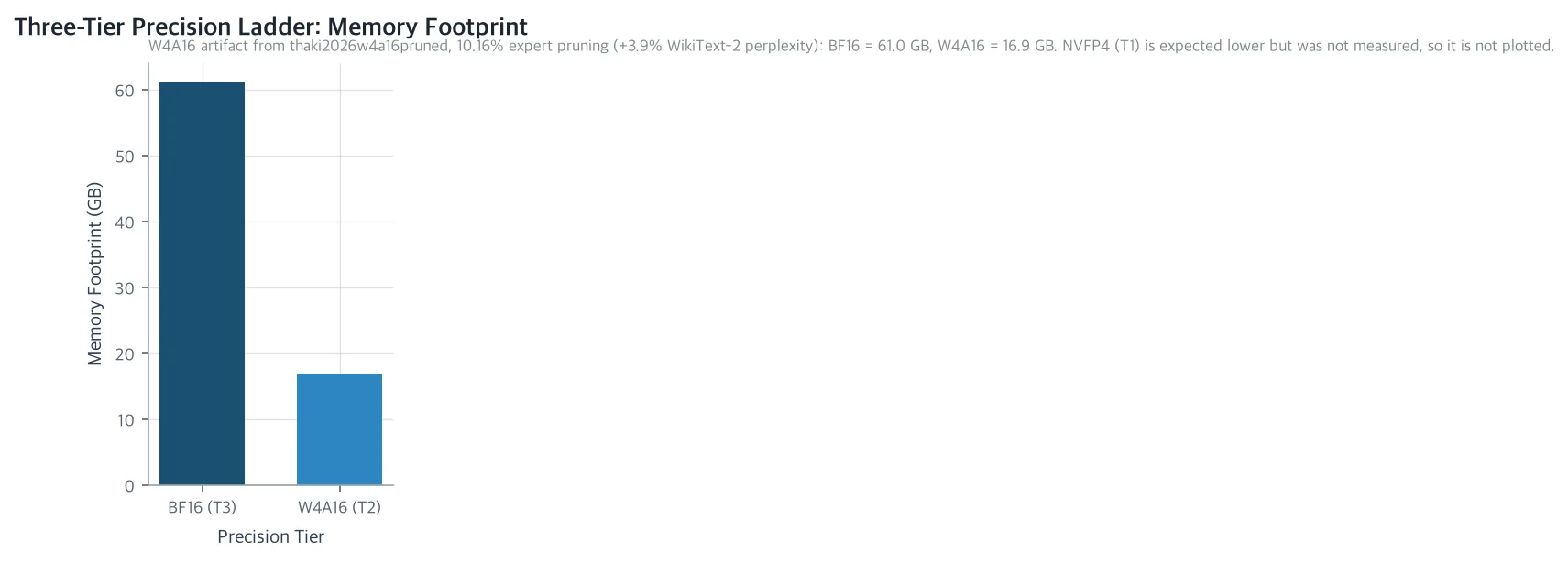The W4A16 compression ratio actually measured on Qwen3-Coder-30B-A3B. BF16’s 61.0GB drops to 16.9GB under W4A16, roughly a 3.6x reduction. This W4A16 artifact also includes a result from pruning 10.16% of experts, so the number is not a pure precision-only change, and NVFP4 was not directly measured in this analysis, so it is not shown on the chart.

How Much Do You Save

The paper formalizes this as a constrained optimization that minimizes expected cost subject to an accuracy floor alpha. In dual form, this is equivalent to maximizing expected accuracy under a cost budget B, and both are tied together by a single Lagrange multiplier, tracing the same Pareto frontier.

To show precisely under what conditions these savings grow larger, the paper uses a simplified two-type model of requests. Easy requests arrive with probability p, and hard requests arrive with the remaining probability 1-p. Easy requests suffer only a small accuracy loss epsilon even at the cheapest tier, while hard requests suffer a much larger loss delta. Because delta is larger than epsilon, any additional budget is always spent optimally by moving hard requests up to a pricier tier first. The resulting routing frontier is a piecewise-linear concave curve with exactly one kink, and this curve is always at least as good as, and usually better than, the straight line traced by a static-split policy that simply mixes a random slice of traffic into the pricier tier.

The maximum savings is given by the following formula:

ΔC* = p(1-p)(δ-ε) / (pε+(1-p)δ) × Δc

What this formula says is clear: savings scale with the variance of the difficulty distribution, p(1-p), and with the gap between the two loss types, δ-ε, and vanish to zero if traffic skews to either extreme (p near 0 or near 1). In other words, if traffic is already homogeneous, there is nothing to route, and the paper presents this as an honest pre-check for whether it is worth building this technique at all. The savings calculation also uses, as its comparison baseline, not the top tier but the cheapest uniform tier that already meets the operator’s accuracy bar, a device meant to avoid crediting routing for gains you could already get simply by lowering global precision, with no routing at all.

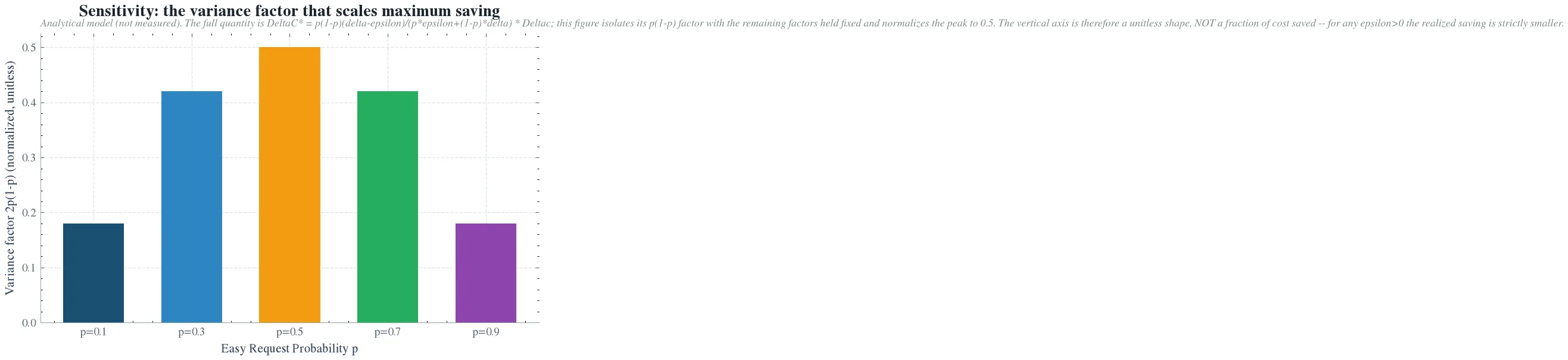A plot of only the p-dependence pulled out of the savings formula above; this is an analytical model, not a measurement. The bars show the normalized variance term 2p(1-p), which peaks at p=0.5 and vanishes at both extremes. The y-axis is a unitless value showing shape only, not a savings ratio, and when epsilon is greater than zero, real savings will always be smaller than this.

What This Means for ThakiCloud and the Wider Community

From the company’s perspective, this result connects directly to the execution economics of Metis, our AI Inference layer. Serving cost is ultimately the foundation that determines how cheaply each piece of work Paxis automates can actually run, so research that structurally lowers per-token cost lifts the execution reliability and economics of the entire Paxis workflow. This paper directly reuses, as one rung of a ladder, the output of ThakiCloud’s earlier work on router-aware selective NVFP4 quantization and on memory-lightweight W4A16 quantization for a pruned 30B MoE model. In other words, parameter-level quantization research and request-level routing research build on each other along different axes, and this paper is the result of extending that axis to a serving policy.

Socially, producing an answer of the same quality with less GPU time and bandwidth means less energy consumed per inference, and it moves in the direction of making it possible for operators without deep capital to host strong open-weight models, since the biggest obstacle to serving a 30B-class model is usually not the weights themselves but the ongoing cost of the accelerator that keeps them running.

Scientifically, what this paper adds to the routing literature is not the credit for first proposing a precision axis (that belongs to prior work adjusting precision at the step level), but the combination of request-level granularity, a K-step ladder, and an analytical Pareto-frontier characterization. In particular, the methodologically clearest contribution is that by explicitly assuming all tiers share parameters, it removes the model-capability confound that has always been baked into the existing cross-model cascade literature.

Limitations

This paper positions itself as an analytical, position paper and has not yet performed empirical validation against actual H200 serving traffic. The only measured number in the paper is the single compression ratio showing W4A16 dropping from 61.0GB to 16.9GB, and the paper itself notes that even this comes from an artifact where 10.16% of experts were pruned, so it is not the result of changing precision alone. That is, the 3.6x figure is only an upper bound on the compression attributable to precision, not an exact measurement of the precision effect itself. Most of the other numbers in the body, including p, delta, and epsilon in the savings formula, are illustrative parameters used to explain the analytical model, not values observed on real traffic.

The accuracy of the difficulty classifier itself has also not yet been measured. The paper explicitly warns that a false-negative rate, where hard requests are mistakenly sent to the cheap tier, actually works in the operator’s favor from a cost-saving standpoint, meaning there is a structural incentive for margin-pressured operators to quietly raise this false-negative rate. The two-type simplification of request difficulty is also a coarse approximation of what is, in practice, a continuous distribution, and the validation case is limited to a single coding-specialized MoE model, leaving open whether the same conclusions transfer to other architectures or workload distributions.

The paper’s detail page is available here: https://huggingface.co/datasets/thaki-AI/daily-paper-2026-08-08-precision-tier-llm-routing