The Precision Ladder: The Cost-Quality Frontier for Choosing Model Size and Quantization Precision Together in Self-Hosted Serving

The reader of this post serves unattended agents on self-hosted GPUs, or is a cloud or AI engineer responsible for the bill of that serving. When you call a model over an API, there was one axis to choose: the model tier. The FrugalGPT-style 1D cascade, where you try a small model first and step up when the quality gate is not met, was the standard design. When you drive your own single GPU, there are two axes. Model size: 4B, 8B, 14B, 27B. And weight precision: BF16, FP8, NVFP4. The node bills the same GPU-time unit no matter which combination sits on it. ThakiCloud’s paper, the “precision ladder,” solves this 2D problem in closed form. It gives a rule for picking the cheapest (model x precision) combination per category, and it predicts the category-by-category reversal routing table where easy categories take small full-precision and hard categories take big 4-bit.

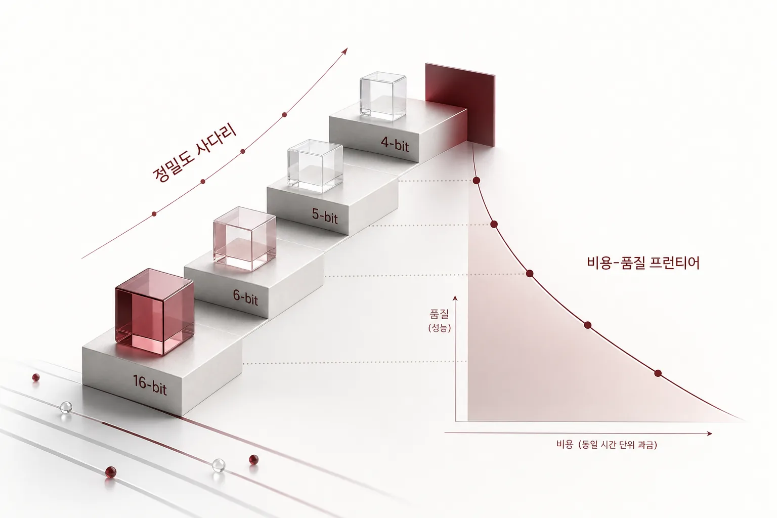A visual metaphor for the article’s key idea.

In Plain Terms: A Taxi Versus Your Own Car

An API is like a taxi fare. Bigger models raise the token rate, a price ticking up on the meter. That is why the step of “try the small model first, escalate to the big one if it fails” matched the cost structure exactly. The FrugalGPT cascade is a design built on top of that taxi fare table.

Your own car is different. The fuel bill runs at a constant per-hour rate no matter which engine it has. A big model shrunk to 4 bits and a small model at full precision burn the same fuel at the same time. The lever on cost is no longer which model you called, but how many tasks you finish per unit of fuel.

The paper compresses this question into a single number. Effective passing throughput E, namely tQ/l. It is the decoding token throughput t multiplied by the code grading pass rate Q and divided by the expected output tokens l per call: the number of tasks per unit GPU-second that pass the quality gate and get delivered. The larger E is, the smaller the bill C per successful task, the GPU-time rate p_h divided by E. In this formula, p_h is the same whichever model sits at whichever precision. The price axis collapses, and the only variables left to choose are t, Q, and l.

The Problem: A 1D Cascade Misses One Axis in Self-Hosted Serving

A FrugalGPT-style cascade stands on two premises. The first is the structure where a quality classifier escalates requests to higher tiers. The second is the API price structure where the call price itself is proportional to the tier. Move to a self-hosted single node and the second premise disappears. Whether you run BF16 4B or NVFP4 27B, the bill is the same GPU-time unit.

The cascade therefore shrinks to following a single row of the 4x3 grid, the BF16 row. The paper’s weak dominance theorem gives it: the cost of a 1D cascade that chooses only within the BF16 row is always equal to or more expensive than the 2D frontier that chooses across the whole grid. The only tie happens when no combination outside the BF16 row is superior in E.

Recent measurements were all 1D. Quantization cliff measurements with the model fixed and only the bit width varied, tier routing with the model fixed and the per-request precision chosen, skill versus model routing with the precision fixed, sampling policies with the model fixed. Only the combined cost-quality frontier of (model size x quantization precision) was still open.

That is why the deployment question this paper answers is clear. For each of the three BFCL-style categories, simple, parallel, and agentic, what is the cheapest (model size x precision) combination that holds the quality gate g=0.85. And is there a category where 27B NVFP4 is cheaper than 8B BF16 per successful task.

The Core Contribution: The Crossover Condition and Byte Parity

The central theorem of the ladder: the crossover condition. The necessary and sufficient condition for a big low-bit challenger (m’, q’) to be cheaper per successful task than a small full-precision incumbent (m, BF16) in a given category is rho_c^t x rho_c^Q > rho_c^l. A product comparison of the throughput ratio rho_c^t, the quality ratio rho_c^Q, and the expected length ratio rho_c^l. If the challenger spits out tokens faster, has higher quality, and produces shorter output, it gets cheaper even with three times the parameters. Expanded to the true bill per successful task, the success rate ratio rho_c^r multiplies the left side one more time.

In the shared regime where the expected length ratio is 1, the condition simplifies further. Writing the quality gap as the product of the tier dividend D_c relative to the BF16 baseline and the quantization cliff tax xi, the condition needed for the crossover is D_c > xi/(1-xi). If the dividend, how much better the big model is than the small one at full precision, is larger than the quality tax that 4 bits erases, big low-bit wins.

There is a reason that condition tilts differently in each category: byte parity. In single-node serving where decoding is the bottleneck, token throughput is set by the rate at which weight bytes are read. 8B BF16 is 2 bytes per weight, for 16.0GB. 27B NVFP4 is 15.2GB at an effective 4.5 bits, 4-bit E2M1 elements plus one FP8 block scale per 16 elements. Three times the parameters, yet about 5% fewer bytes read per forward pass. That is why the throughput ratio stays near 1, and the paper sets 0.9 to 1.05 as the reasonable prior distribution. When throughput is effectively equal, the crossover condition shrinks to the quality balance, the fight between D_c and xi.

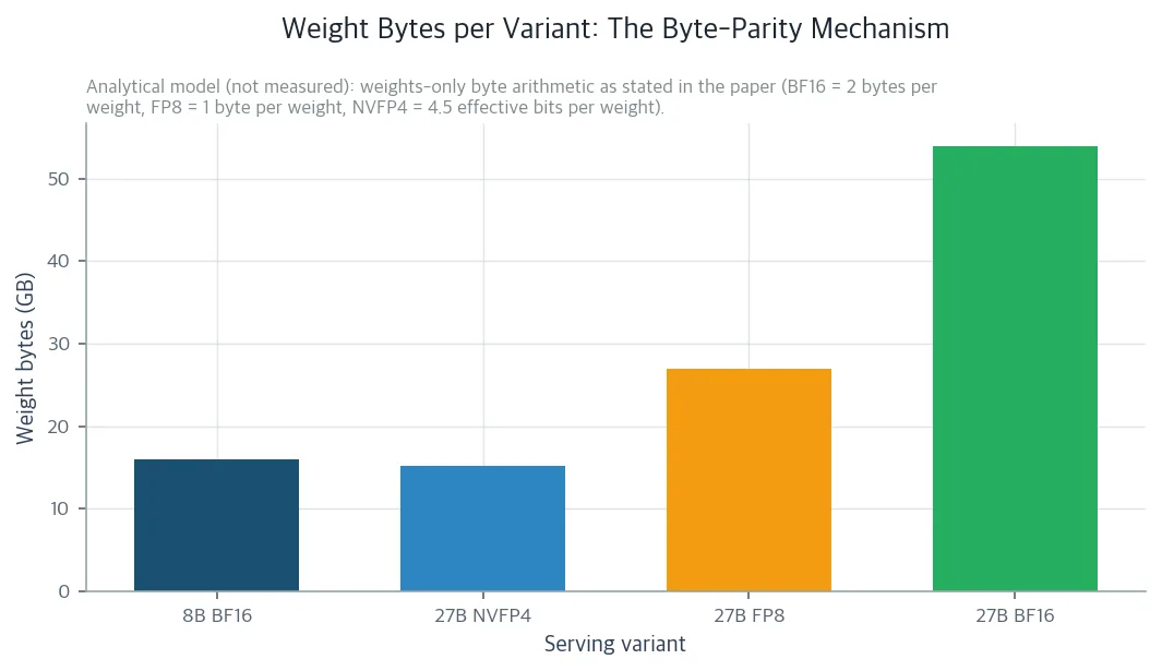The weight byte arithmetic at the crossover point. 27B at an effective 4.5 bits per weight is 15.2GB, 8B at 16 bits is 16.0GB, so the 27B with three times the parameters reads about 5% fewer bytes per forward pass. 27B at FP8 and BF16 are proportional references. (Arithmetic of the interpretive model, not a measurement. BF16 is 2 bytes per weight, FP8 is 1 byte, NVFP4 is computed at an effective 4.5 bits)

The shape of the regime, three branches. In the dividend-dominated regime, (1+D_c)(1-xi) increases with the structural decode depth s_c of the category, and the crossover holds only in the hardest category. It draws the true face of the precision ladder: small full-precision on easy categories, big low-bit on hard ones. In the cliff-dominated regime, every category is below the threshold and the 1D cascade is already the 2D optimum. In the low-bit-dominated regime, big low-bit is optimal in every gate-passing category. Which shape actually emerges is determined by the output of the pre-registered protocol.

It also gives one hardware transfer theorem. Transferring values measured on H100 NVL (93.6GB) to H200 (141GB, price ratio 1.4) leaves the routing table itself unchanged. Absolute dollar cost improves only when the per-category common factor beta_c exceeds the price ratio 1.4, and memory headroom transfers of course. Falsification criterion R4 closes the tolerance of beta_c.

The Worked Example: A Sign Flip Seen With Scenario Values

The calculation below is not a measurement. It uses the scenario values the paper explicitly states, and each assumption is carried over as-is from the context. Shared regime assumption, rho_c^l=1, true success overlay rho_c^r=1. The throughput ratio rho_c^t is 0.95 from byte parity. The quality of 27B NVFP4 is the cited anchor 0.896, the full-suite value over the 800-item BFCL-style suite, assumed category-invariant. The per-category quality of 8B BF16 is set to 0.95 for simple and 0.80 for agentic.

In simple, the quality ratio is 0.896/0.95=0.943. The product is 0.95 x 0.943=0.896, below 1. No crossover. The small full-precision model saturates the easy category, so 4-bit has no room to win even while carrying the cliff tax. The winner of simple is 8B BF16.

In agentic, the sign flips. The quality ratio is 0.896/0.80=1.120, and the product is 0.95 x 1.120=1.064, above 1. Crossover. 27B NVFP4 is about 6% cheaper per successful task. In a structurally hard category, the BF16 quality gap between 27B and 8B, the tier dividend, pays off the 5% throughput gap.

The sign flipping by category means the same 27B NVFP4 is more expensive than 8B BF16 in simple and cheaper in agentic. The paper’s central prediction, the category-by-category reversal routing table, comes straight out of this calculation.

The Feasibility Layer: Memory Was Not the Constraint

The measurement layer is deliberately thin, and that thin layer is what supports the study. On an H100 NVL, 93.6GB node, the BF16 peak VRAM of 4B/8B/14B is 7.5/15.3/27.5GB, so even the biggest 14B only reached 29.4% of capacity.

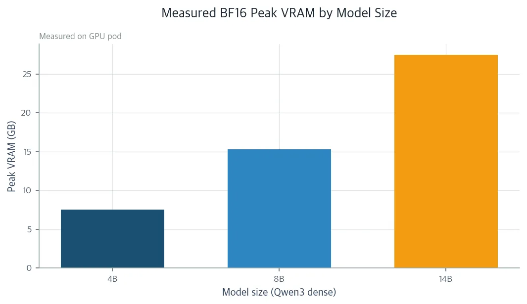Measured BF16 peak VRAM of the Qwen3 4B/8B/14B checkpoints on a 93.6GB node: 7.5/15.3/27.5GB, leaving over 70% headroom, so the constraint on the feasible set was the stack, not memory. (Measured in the GPU pod)

That leaves 66.1GB, over 70% of headroom. Extending the byte parity arithmetic to the 27B row gives BF16 54.0GB, FP8 27.0GB, NVFP4 15.2GB. The entire 4x3 grid fits on 93.6GB. There is no need to argue about the 141GB of an H200.

Checkpoint loading time grows smoothly from 2.2 seconds for 4B to 5.0 seconds for 14B. The parallel download of the three checkpoints was all around 171 seconds, and the total wall time of the feasibility pass was 189.8 seconds.

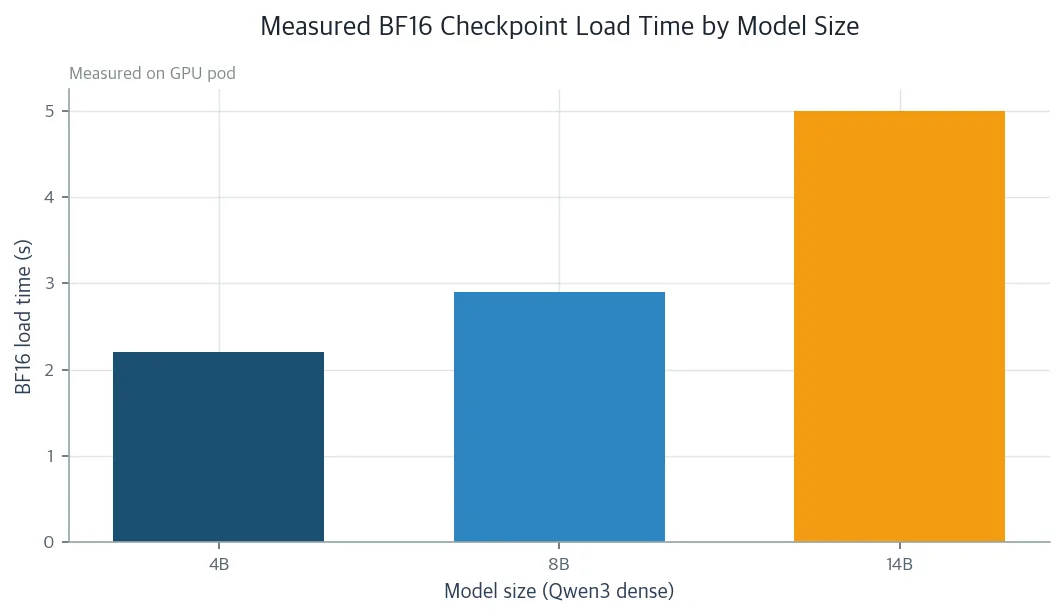Measured BF16 checkpoint loading times on a 93.6GB node. They grow smoothly from 2.2 seconds for 4B to 5.0 seconds for 14B. The total wall time of the feasibility pass was 189.8 seconds. (Measured in the GPU pod)

The decisive constraint was the stack, not memory. Six attempts at the 8-bit and 4-bit nf4 loading paths of bitsandbytes, three sizes x two precisions, all failed. In this stack, the only usable low-bit axis is the framework-native quantized checkpoints, namely NVFP4 from the production serving stack. The feasible set F is determined by stack support, not memory.

Price and quality anchors are cited inputs. GPU-hour rates: H100 $2.50, H200 $3.50, B200 $5.00, RTX 5070 $0.60. The H200/H100 ratio is 1.4. The quality anchor is 89.6% on the 800-item BFCL-style suite for the 27B NVFP4 production checkpoint (2026-09-06).

The Validation Design: The Pre-Registered Protocol and Falsification Criteria R1-R4

The quality-throughput values of the grid cells are designated as the output of this protocol. The workload is 24 items in total: 12 simple, 8 parallel, 4 agentic. Token budgets are 96 for simple, 192 for parallel, 128 for agentic. Single-call categories use a fixed budget with EOS disabled, and agentic uses a per-turn cap. The throughput probe is taken at concurrency C=8, N=64 sequences.

Three falsifiable predictions. P1, non-degeneracy of the ladder: two or more of the three categories pick a different combination. P2, cascade crossover: in at least one category, a low-bit point outside the BF16 row is optimal. P3, category-by-category reversal: 27B NVFP4 beats 8B BF16 in agentic but not in simple.

Falsification criteria R1-R4 close the other side. R1: if the per-category quality of 8B BF16 exceeds 27B NVFP4 quality x throughput ratio in every category, the headline crossover is invalid in every category. R2: if the BF16 row dominates in every category, that means the precision axis itself is redundant under the gate. R3: if the 8-bit to 4-bit tax jump does not exceed the 16-bit to 8-bit increment, the superlinear cliff prediction is refuted and the ladder threshold is re-derived under linear cliffs. R4: if H200 measurements deviate from the H100 NVL model by more than 20%, the hardware transfer theorem is refuted.

What the Company, Society, and Science Get

What remains for the company is a deployable routing table. One per category: the (model x precision) combination that maximizes E while holding the gate g=0.85. Since the only low-bit point with a current cited anchor is 27B NVFP4, the first rung of the ladder is pinned to that point. Categories where the crossover test holds against the BF16 incumbent take 27B NVFP4, and categories where it does not hold keep the FrugalGPT-style BF16 row.

This table occupies one stage of the four-stage combination of the token factory. The zero-token skill router sends skills by category. The routing table assigns categories to rungs of the ladder. The post-verification retry of the free deterministic validator owns the number of draws inside the endpoint. The queue-aware tier fallback descends to the next rung under queue pressure. The four factors of the bill, the hardware rate p_h, the length policy l, throughput t, and quality Q, are each owned by one of the four stages. If any single lever changes, the bill rescales in place and the rest of the structure is left untouched.

It also holds at this point that the retry does not affect the bill. Under the free deterministic validator, the expected number of draws per passed task is exactly 1/Q, and the retry budget moves only the give-up rate. The direction of fallback is also by E order, not by size order. A smaller low-bit rung that leads in E is a legitimate fallback destination before the bigger BF16 rung.

For society, this is the point where the dollars and electricity of unattended automation shrink. When it is quantified at what cost big low-bit matches small full-precision quality, self-hosted serving operators get a concrete recipe for cutting inference spend per task.

For science, this is the point where the FrugalGPT-style 1D cascade is promoted into the 2D cost-quality frontier of (model size x quantization precision). Including, in agent tool-calling workloads, the interaction with the per-category low-bit accuracy drop, namely the tool-calling cliff. The crossover condition is in closed form, and the FrugalGPT cascade is absorbed as the BF16-row projection of this frontier.

The Parts You Should Not Trust

This paper is an interpretive study. The measurement layer focuses on feasibility, and the grid-cell quality and throughput values are not new measurements. The scenario values of the worked example, the per-category quality of 8B BF16 at 0.95 and 0.80, are assumptions.

The first boundary is a single Qwen3 dense family. Transfer to MoE families or other families is open. In MoE, routing-aware quantization matters especially. The second boundary is hardware transfer. The measurement is on H100 NVL and the deployment target is H200. The transfer theorem is conditional: absolute dollar cost improves only when the common factor beta_c exceeds the price ratio 1.4. R4 watches that error.

The gate is also fixed at a single point, g=0.85. Other operating points can be re-derived in the same closed form, but they require a protocol re-run. Keep the shared regime assumption in mind too. rho_c^l=1 means no length inflation, and if low-bit inflates reasoning tokens or silent errors grow in compressed models, rho_c^l>1 or rho_c^r<1, the required dividend rises, and the crossover set shrinks. A conservative direction, but read the inequalities under that light. Prices are also public on-demand list prices. Even if spot or preemptible pricing, or internal power costs, change the level of p_h, by Lemma 1 the order of the ladder itself cannot move.

Finally, the regime that actually materializes still has no answer. Which of the three branches, the ladder, the empty crossover, or low-bit dominance, emerges comes after running R1-R4. But the point where the sign must be wrong is already fixed. You can just read along with the protocol that closes that result.

Paper and data: https://huggingface.co/datasets/thaki-AI/daily-paper-2026-09-27-precision-ladder-model-quant-routing