KV Cache Tiering and Prefill-Decode Disaggregation Together: Does H200 MoE Serving Cost Actually Drop
This post is useful both for teams disaggregating prefill and decode into separate serving pools and for teams using tools like LMCache to tier KV caches off the GPU to raise reuse rates. Both techniques have been validated on their own, but what happens when you combine them has barely been examined. The paper covered here structures that combined effect mathematically, then reports honestly on an attempt to actually measure it on an H200 cluster, an attempt in which the vLLM engine died twice. The short version: combining the two techniques is not always a win, and which side wins is determined not by hardware but by the workload’s reuse pattern.
 A visual metaphor for the article’s key idea.
Two Optimizations: Splitting Prefill From Decode, and Stacking the Cache Into Tiers
LLM serving cost is shaped by two stages with fundamentally different characters. Prefill processes the entire prompt at once to fill the KV cache, a compute-intensive burst of work; decode keeps reading that cache and the model weights to emit tokens one at a time, a memory-bandwidth-intensive workload that runs for a long stretch. When both run in the same GPU pool, a single batching policy has to satisfy two conflicting goals at once (time to first token and per-token latency), and both end up worse off. Prefill-decode (P/D) disaggregation, as proposed by DistServe, solves this by splitting the two stages into independent GPU pools and moving the KV cache between them.
Tools like LMCache go after a different kind of waste. Building on top of the block-level KV management that vLLM’s PagedAttention introduced, they push KV blocks that previously lived only in GPU memory (HBM) out through a tier that continues into host DRAM and local disk, so the cache is not discarded once a request finishes and can be reused later. The problem is that these two techniques touch each other’s assumptions. When prefill and decode sit on the same GPU, the KV that prefill just produced is already sitting in the HBM that decode is about to read, so tiering only helps with reuse across requests. Once the two are disaggregated, the decode worker does not hold that KV at all, so every request has to pay a transfer cost, and a tier lookup stops being something you consult when there is slack and becomes a critical path that sits directly on the latency budget. Because of that, this paper does not simply add the two techniques together; it first works out what actually happens when they are combined, using an analytical model.
Disaggregation Raises the Cache’s Value While Disqualifying the Slowest Tier
There are two core observations, and they point in opposite directions. First, a disaggregated prefill pool merges caches that used to sit separately on each server into a single logical domain. There is no longer any need to duplicate a popular prefix across servers, so the more skewed the reuse distribution is (the heavier its tail), the more the hit rate rises even at the same capacity. In other words, disaggregation raises the value of tiering. Second, time to first token (TTFT) has a service-level target, and within that target there is only so much slack available for a cache lookup. The transfer time that disaggregation introduces eats directly into that slack, and because bandwidth differs so sharply across tiers (as shown below, HBM and NVMe differ by roughly 1,600x), the slowest tiers are the first to fall off the critical path. Disaggregation makes the cache more valuable, but the very tier that would realize the most of that value becomes unusable for exactly the same reason.
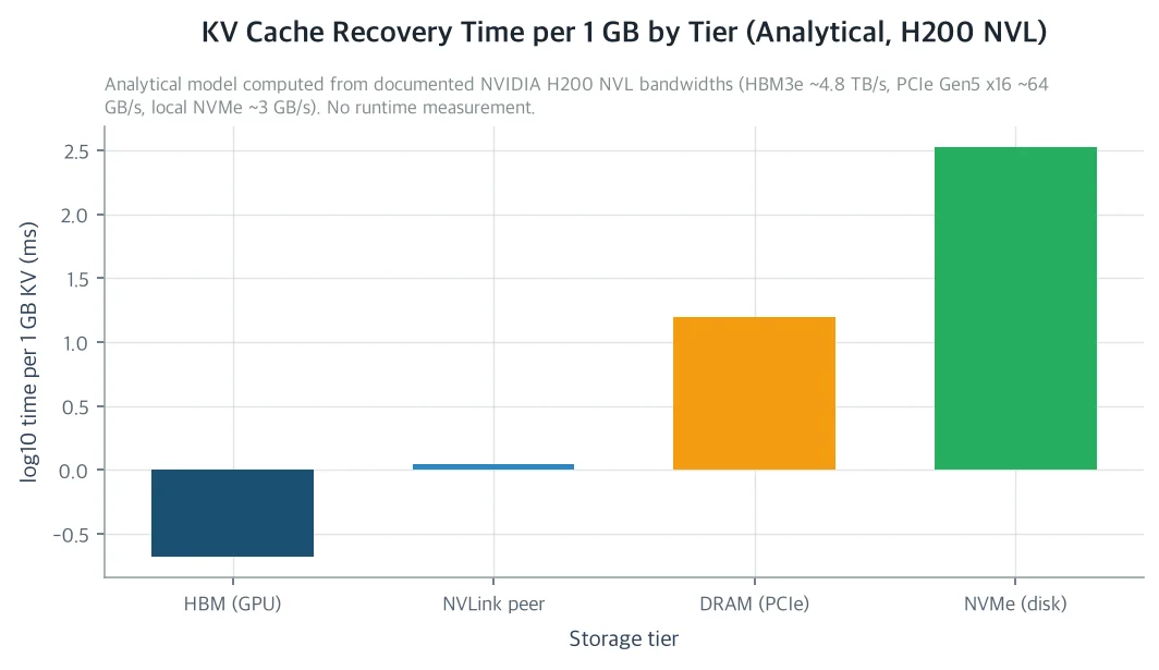 An analytical model computed from published H200 NVL hardware specs (not a measurement). The chart compares, on a log scale, how long it takes to recover 1GB of KV cache from each tier. HBM takes roughly 0.21 milliseconds and NVMe roughly 333 milliseconds, a gap of about 1,600x, and this gap effectively determines which tiers can remain on a latency-sensitive path.
The paper also attaches concrete numbers. For a typical configuration (32 attention layers, 8 KV heads, head dimension 128, 2 bytes per element), KV bytes per token work out to roughly 130,000 bytes, meaning a prefix of about 8,000 tokens corresponds to 1GB of KV cache. HBM recovers that 1GB in under a millisecond, while NVMe takes nearly a third of a second, so within a typical TTFT target measured in the low hundreds of milliseconds, the transfer alone already exhausts the slack, and the disk tier is automatically disqualified from the critical path. The conclusion that follows is that the disk tier should be demoted from something you query synchronously to an asynchronous prefetch target that gets pulled into DRAM ahead of time. Because the two observations point in opposite directions, the net effect depends on whether the workload is bound by hit rate (synergy) or bound by slack time (cancellation).
A Break-Even Formula for Deciding Whether Another Tier Is Worth Adding
The practically important question here is how much capacity to invest in the DRAM or disk tier. The paper assumes the reuse distribution follows a heavy-tailed power law, and, working from the premise that each additional unit of capacity yields a diminishing gain in hit rate, derives a break-even capacity. The benefit of adding each extra byte is the prefill recomputation cost it saves; the cost is the rent of keeping that byte around. Setting the two equal yields an economically optimal capacity for tier t that scales as a power of 1/(1-beta) in the reuse distribution’s tail exponent (beta); as this exponent approaches 1 (meaning reuse is spread more evenly), the required capacity explodes superlinearly.
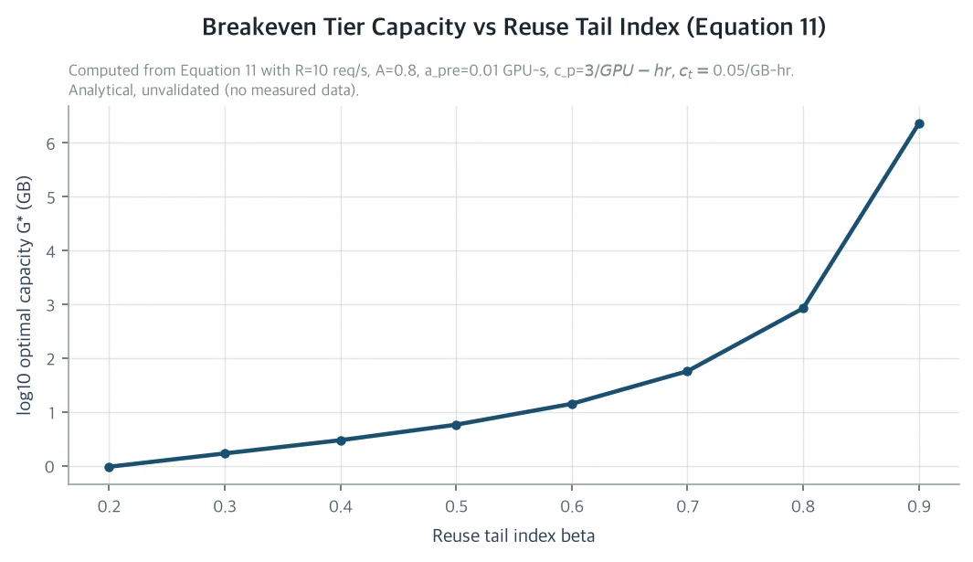 An analytical model computed by fixing example values for request rate, prefill recomputation cost, GPU unit price, and storage rent (not a measurement). It shows that as the reuse tail exponent beta approaches 1, the break-even capacity rises steeply even on a log scale.
The implication of this sensitivity is clear. Tiering capacity is driven far more by the nature of the workload than by the hardware, so even on the same H200 cluster, the DRAM and NVMe capacity two different services need can differ by more than an order of magnitude, and provisioning guidance derived from one deployment cannot simply be carried over to another. Moreover, this optimal capacity has to be checked against the slack-time constraint described earlier, independently. If disaggregation has been pushed aggressively enough that slack is already tight, no matter how large a capacity the break-even formula justifies, the disk tier still cannot sit on the critical path, and the only option left is a two-tier setup where that tier is relegated to prefetching.
The vLLM Engine Died Twice When We Tried to Measure This on H200
Everything up to this point is the analytical model, and the paper’s original goal was to layer a measured latency-cost curve on top of it to inform provisioning for the Metis inference serving stack. On July 27, 2026, the team actually attempted to validate this on a single H200 NVL GPU on the internal H200 cluster (tkai-prod-compute-h200, node tk-ai-wkld-wk-gpu-003). To confirm the harness, the image, the LMCache connector, and the metrics-collection path all worked before spending GPU hours on an MoE sweep, they chose a small dense model (Qwen2.5-0.5B-Instruct), not an MoE model, as a canary. The weight download finished normally in 148.7 seconds, but the vLLM engine core initialization that followed failed. Twice. Once with an option enabled that hard-caps the KV block budget, and once with that option turned off on retry, and it failed identically both times.
The error message took the form “engine core initialization failed, see above for the root cause,” but the log line that actually held the root cause sat in an engine-internal log stream the harness had not captured, and the list of failed core processes was reported empty. The actual cause could not be pinned down, and not a single performance sample, latency, throughput, or cost, came out of the run. Searching public vLLM issues turned up this exact same message recurring across at least four unrelated issues (checkpoint mismatches, GPU memory or cache block exhaustion, tensor-parallel configuration problems, and platform-specific bugs), which means the exception text itself carries almost no diagnostic value; it does not distinguish between causes. The team also floated a hypothesis that the hard KV block budget cap might have conflicted with the LMCache connector’s tier-sizing plan, but the fact that the retry without that option failed the same way undercut the hypothesis on its own, so the paper leaves it as an unconfirmed hypothesis rather than a conclusion. Following the precedent set in an earlier dynamic-batching tuning report, where a narrow null result was reported as-is, the team again reported the failure itself as the result rather than filling in the gap with substitute measurements.
What This Paper Leaves for the Company, for Society, and for Science
For the company, the practical value of this paper is not a performance number but a decision framework and a warning sign. The break-even formula and the slack-time constraint give the Metis inference serving team grounds to size DRAM and NVMe tier capacity from our own reuse distribution rather than vendor claims. And the experiment failure is itself a warning. The startup-time contract between the engine’s memory-sizing configuration and a third-party KV connector’s tier-planning logic turned out to be a genuinely fragile and hard-to-observe failure point, and this incident confirmed directly that a canary validation with full log-stream capture is a prerequisite before any serious capacity investment.
Socially, GPU time wasted on KV cache recomputation is real energy waste, and lowering the cost per token makes LLM inference more accessible to smaller organizations. That effect is conditional, though. Tiering only lowers cost when the break-even condition is met; over-investing past that point just trades one kind of waste for another. So the public-interest message this paper offers is less “turn tiering on unconditionally” and more “measure your reuse distribution before you invest.”
Scientifically, it fills a gap: the prefill-decode disaggregation literature and the KV cache tiering literature have each matured on their own, but no work had examined the two together in a single variable space. It explicitly shows that two opposing forces coexist, disaggregation raises the cache’s value while lowering the availability of the slowest tier, and it presents the fact that the balance point is set by the workload’s nature (the reuse tail distribution) rather than by hardware, as a new axis added to the cost-latency Pareto frontier discussion.
Limitations, and What to Check Next
The paper’s most fundamental limitation, as already stated, is that it has not a single measured value for either performance or cost. The model’s assumption of a power-law reuse distribution could also break down: if the real workload is non-stationary, with the set of popular prefixes shifting over time, the tail exponent itself would shift and the precise form of the break-even formula could fail to hold. Even had the experiment succeeded, the model chosen for validation was small and dense, so it would not have reflected MoE’s cost structure at all, and the single-GPU setup means the transfer-cost terms that disaggregation introduces would not have been validated either. The vLLM issue diagnosis was also not reproduced directly; it draws on public reports, so it should be interpreted narrowly and with caution.
The paper lays out the next steps in specific order. First, fix the harness to capture the engine’s child-process logs in full and pin the image tag to secure reproducibility. Next, run a 2x2 experiment crossing the KV block budget option with whether the LMCache connector is enabled, to narrow down the real cause of this failure; measure each tier’s fixed overhead directly across varying prefix lengths; and run actual production prompt traces through a cache simulator to estimate the reuse distribution’s tail exponent offline, without a GPU. Only after these four steps are done would the team run a sweep across prefill-decode ratios and tier configurations with an actual MoE model and a multi-node setup, obtain the latency-cost frontier, and report how far it diverges from this paper’s analytical formulas.
You can find the full paper here: https://huggingface.co/datasets/thaki-AI/daily-paper-2026-07-28-kv-cache-tiering-pd-disagg-cost