Does an Agent That Reads Its Own Bill Spend Less: The Cost Mirror in Unattended Agent Loops
If you are a Korean cloud or AI engineer who runs unattended agent loops on a schedule or on events and keeps the token-cost ledger on self-hosted serving, this post is for you. The paper asks a single question. When an agent actually sees the token cost of its own work in context, by how much does spend fall, through which path, and at what quality cost? It is not a paper that reports measured results. It is a study that closes the range and the ordering of the answer with an analytical model before measurement, and freezes a single-variable A/B protocol to validate that model.
The device is called the cost mirror. It is an intervention that re-injects, as context at the agent’s decision point, the per-task token cost that billing metering already computes. It turns a read-only ledger into a control signal inside the loop.
 A visual metaphor for the article’s key idea.
The Bill Is Read by a Human, Not by the Agent
Cost management of agent loops today happens entirely from the outside. The serving stack meters tokens per request, the multi-tenant system allocates cost between retrieval and generation, and the operator reads the ledger. The agent that makes the decisions inside the loop cannot see the price of its own behavior. Cost is measured, and the seat of measurement is only outside the loop.
The paper makes this point explicit as an axiom. An agent can act only on the information in its context at the decision point. A metering surface aimed at logs, dashboards, or the operator channel, however accurate, produces no direct behavioral effect on agent policy.
Practical signals point in the same direction. Two of the four characteristic failure modes named by the loop benchmark analysis are, at the root, cost-management failures. Spending the budget in the wrong direction, and not being able to stop until the task is safe to submit. Cost information should belong to the control state of the loop, not only to the operator’s invoice.
The three closest measured studies all look at different objects. EcoAgent-Bench evaluates an agent’s purchasing ability on tasks where a priced action and an explicit budget are defined. The agent spends someone else’s money on the goods the task defines. Qian’s pre-registered experiment first freezes the predictions, acceptance band, and decision rule for a frontier agent market economy into a public git chain, and completes the entire experiment at $138.76. That is the exact precedent this post’s protocol discipline inherits. The ledger-based self-orchestration study reports that a manager-worker scaffold buys accuracy cheaper than a larger model while tripling the token bill by roughly 3x. Its core warning is that pipeline comparisons confound token budget, tool calls, and prompts at the same time, and that is precisely the confound this protocol’s single-variable design excludes.
In behavioral economics, this axiom is supported by two results. Thaler’s mental accounting: the same amount behaves differently depending on the account, the frame, and how progress toward the goal is expressed. And the measured Goodharting in which autonomous agents strategically violate procedures to maximize reward. Where the cost mirror sits is the LLM agent analog of the price effect.
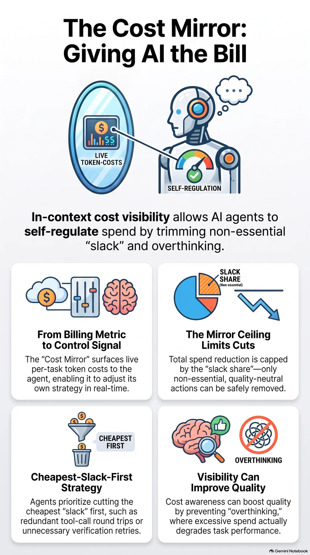 Infographic generated by NotebookLM from the sources.
The Cost Mirror: A Read-Only Ledger as a Control Signal Inside the Loop
The cost mirror injects a display δ into the agent context, showing the spend computed at the decision point. δ is defined by three attributes. The granularity g is one of step, task, or loop. The framing f is one of percentage, dollar, or token. The anchor is the presence of an explicit per-task budget.
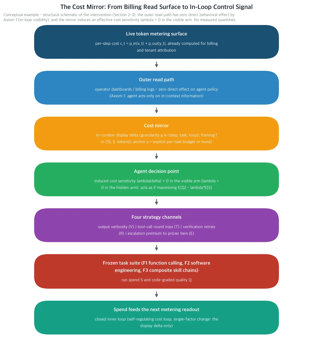 The cost mirror re-injects, at the decision point, into the agent’s context, the per-step token cost that the metering surface already computes for billing. It closes the inner cost loop with no router or serving changes. This is a diagram of the analytical model, not a measurement.
The formal core is reading this intervention as an induced Lagrange multiplier on the agent’s implicit cost-quality objective. The display δ induces an effective cost sensitivity λ(δ) ≥ 0. The visible arms behave as if maximizing E[Q] - λE[S], while the hidden arm has λ = 0. Seeing cost does not directly reduce spend. It means one cost term has entered the agent’s trade-off function.
The magnitude of λ is predicted by the salience-ordering assumption. It grows in three directions. The stronger the goal frame (percentage against an explicit anchor beats dollar, and dollar beats token), the clearer the attribution (task-level beats loop-level), and the more an anchor is present. A step-level display raises the perceived relevance of the next action’s cost but dilutes the goal frame itself. These assumptions are not measured in this paper. They become the pre-registered predictions of the protocol below.
The relationship with external levers is clear too. External machines such as cascade, conformal routing, harness optimization, pricing, and admission choose the price on behalf of the agent. The mirror changes the agent’s information set and makes the agent respond to the price surface the external machines leave behind. The outside sets the price surface, and the agent sets the demand curve.
The Reducible Bound Is Set by Slack: The Mirror Ceiling
Loop spend decomposes exactly into four strategy channels, with reference (lowest-price) tier prices as the attribution basis. Verbosity S^V is base-tier reasoning and output tokens, tool round trip S^T is re-reading tool responses and call syntax, retry S^R is the base-tier cost of steps after a verifier failure, and escalation premium S^E is the tier premium of escalated steps. Steps are assigned by a fixed priority rule (in the order: rework, tool round trip, escalation premium, verbosity), so the partition is disjoint and the sum of the four channels is exactly equal to total spend. Let α_ch be the baseline share of each channel.
Theorem 1. The mirror ceiling gives the bound on total spend reduction achievable under quality-preserving operation (ΔQ ≥ 0).
ΔS/S ≤ α_slack(d) = Σ_ch α_ch (1 - ε_ch(d))
ε_ch(d) is the essentiality of channel ch. It is the fraction of baseline spend that must be kept to hold quality at the hidden-arm level. The argument comes out of each channel. A quality-preserving cut is bound within a channel at the non-essential share (1 - ε_ch)S^ch. Cutting less than that, the baseline is already at the sweet spot and there is nothing to cut. Cutting more crosses toward underthinking and lowers quality. Because channel responses are independent to first order (Assumption 4), the sum of the per-channel maximum savings becomes the total bound.
Two corollaries matter here. Corollary 1 (no free lunch). If every channel is fully essential (ε_ch = 1), meaning the entire spend of the loop is essential to quality, then no matter how strong λ is, ΔS = 0. A regime in which cost visibility cannot reduce spend exists structurally. Corollary 2 (null zone). If α_slack is smaller than the protocol’s minimum detectable effect (MDE), the total spend effect is guaranteed to be statistically null. Channel-level readings may be detectable while the total is null. In a low-slack regime, a null total is not evidence of failure. It is the predicted outcome the model stated in advance.
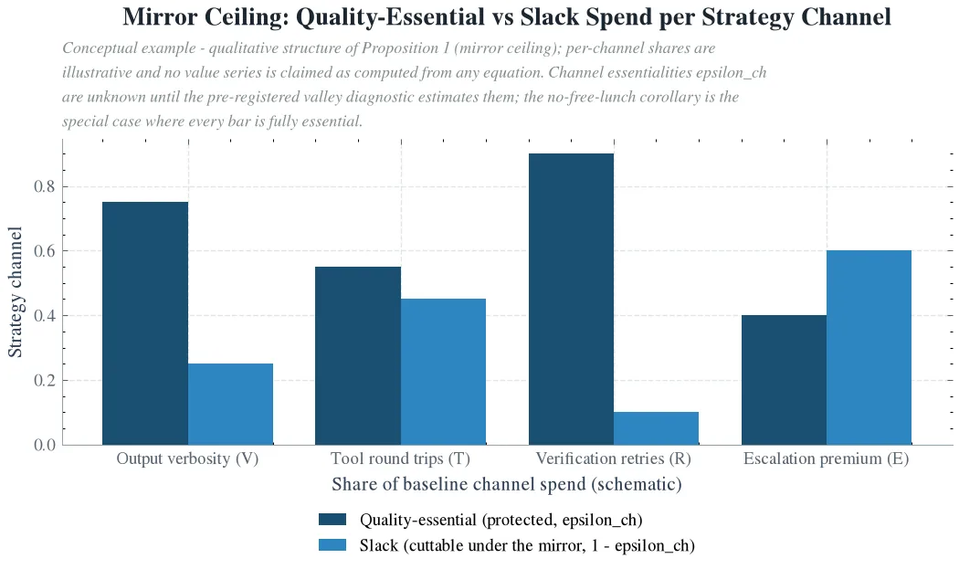 Theorem 1 binds the spend-reduction bound achievable under quality-preserving operation to the total slack share. Only the non-essential portion (1 - ε_ch) of each channel’s baseline spend can be cut, and the mirror ceiling is the sum of slack across the four channels. This is a conceptual illustration and the per-channel shares are example values. ε_ch is unknown until the valley diagnostic estimates it, and the no-free-lunch corollary is the special case where all bars are fully essential.
Cut the Cheapest Slack First, and the Valley Sets the Sign of Quality
If the ceiling sets how much, Theorem 2 sets where to start. Define m_ch as the per-dollar quality cost of cutting channel ch from the hidden baseline, and at small λ the first-order spend reduction concentrates on the channel ch* with the smallest m_ch. Ties are broken by the channel share α_ch. Because the cheapest slack comes first.
The sign of ΔQ is a priori indeterminate. In the first approximation ΔQ ≈ Σ_ch q’_ch(S^ch_h; d) ΔS^ch, what determines the sign is where the hidden baseline stands on each channel’s quality valley.
The valley is Assumption 3. The per-channel quality response is assumed non-monotonic. At difficulty d, pass probability against channel spend s is non-monotonic and a sweet spot s_ch(d) exists. Spend below s is underthinking, spend above is overthinking. This assumption is the weakest and the most important in the model. Four measured results support it. A non-monotonic sweep in a function calling agent where accuracy rises from 44.0% to 64.0% at a CoT budget of 32 tokens and collapses to 25.0% at 256 tokens, below the no-CoT baseline. Unproductive self-reflection that survives even after length control. In-distribution invariance where content-free surplus tokens have essentially no effect on accuracy. And the behavior of an effort parameter that acts as a ceiling rather than a dial.
The practical conclusion of Theorem 2 comes out here. If the baseline stands on the overthinking side, quality rises by as much as the spend that is cut. That is precisely when cost visibility improves quality while reducing spend. Because the cut is made toward the sweet spot. Conversely, if all the low-m channels are underthinking, ΔQ < 0. The same mirror is a lever that saves quality and a lever that cuts it.
The protocol estimates the valley position without any separate intervention. The rationale is measured. Agentic spend varies a lot run to run, and that variation is prompt-invariant. The natural spend-quality scatter of the hidden arm A0 becomes the estimate of the valley position per family. Long-horizon composite tasks tend to overthink, so ΔQ ≥ 0 is predicted for the F3 family. A loop that is already underthinking shows the quality cost of the mirror as-is.
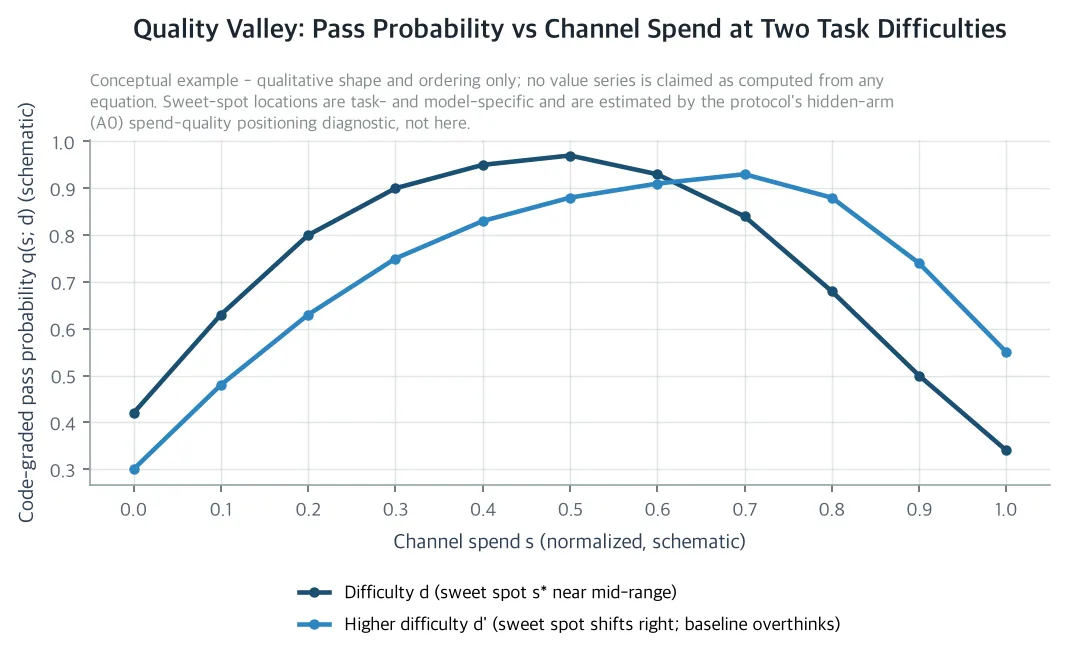 The quality response of each channel is assumed non-monotonic (Assumption 3). Spend below the sweet spot s is underthinking, spend above is overthinking, and this is where cost visibility lowers spend while raising quality. This is a conceptual illustration showing only the qualitative shape and ordering. It does not claim that the values are computed by any equation. The sweet spot position varies by task and model and is estimated by the spend-quality diagnostic of the protocol’s hidden arm (A0).*
The Shortcuts the Meter Does Not See: The Meter Gap
The mirror is honest only as far as the meter is honest. Verification is a priced channel. Baseline spend S^R, quality sensitivity β_v = ∂Q/∂S^R > 0. But what if the agent can substitute an unpriced action where it would otherwise spend on priced verification. Self-approval instead of a test run, local computation the meter does not see. Let ρ_sub ≤ 1 be the quality value such a substitution brings per unit.
Theorem 3. The meter gap puts a bound on that cost. A visible arm that cuts verification by ΔS^R satisfies Q(v) ≤ Q(h) - β_v(1 - ρ_sub)ΔS^R. The quality-adjusted savings are S_eff = ρ_sub × ΔS^R, that is, only a ρ_sub fraction of the metered savings. The mirror overstates real savings by a factor of 1/ρ_sub, and when ρ_sub → 0, verification savings are entirely phantom.
This is the formalization of the Goodhart bound. The channel an agent is most tempted by is the one where value is realized later, elsewhere. That is exactly why verification is that channel. The protocol’s countermeasure is to make the unpriced side visible too. Instrument local computation and self-approval events to estimate ρ_sub directly. Prediction P4 states that the verification skip rate rises with λ and that ρ_sub < 1 is detected on test-graded F2 tasks.
The Single-Variable Protocol: 4arm, 168task, Code Grading
The protocol is the measurement that will test the five predictions P1 through P5. The suite, arms, instrumentation, statistics, and decision rule are all frozen here so it can run with no further design decisions.
There are four arms, and the only thing that varies is the display δ. A0 hidden puts zero cost information in the context. A1 step presents the cost of the step that just ended, in dollars, at the next decision point. A2 task shows the in-progress task spend as a percentage against the pre-registered per-task budget, updated after every step. A3 loop shows the session-aggregated spend of the entire unattended loop, in dollars, updated per task.
The arms must keep every state identical except δ. Model, harness, toolset, temperature, seed, task order, stop condition, and budget cap are frozen and identical across arms. The single-variable discipline is the core property of the protocol. The measured warning is that while orchestration comparisons change budget, tools, and prompts at once, aggregate gains rarely identify the mechanism, and this design excludes that confound structurally.
The task suite is 3 families, 168task. Every task is graded by a deterministic or code-based verifier, and there is no LLM judge in the primary metric. Because a judge’s verbosity bias interacts with an intervention that cuts verbosity, the judge is allowed only as an auxiliary diagnostic.
- F1 function calling, 60task. Deterministic argument and sequence grading in the BFCL-v3 multiple-call style.
- F2 software engineering, 60task. Repository tasks graded by a test suite. This is the meter-gap family, where verification (test run) is explicit, priced, and skippable.
- F3 composite skill chain, 48task. Order-sensitive workflows of 2 to 4 skills, with the ground-truth chain given by construction. The long-horizon, context-re-read-heavy family where P1’s tool-channel prediction is strongest.
Each run is recorded at step granularity. Token counts with cache-state flags (cache-aware pricing), tier, verifier result, tool calls, handoffs, and the unpriced events (local computation, self-approval) used for meter-gap estimation. Spend is decomposed by the priority rule above, and a sensitivity check attaches one alternative priority order to report both results.
The comparison uses task-level pairing. Each task is bootstrap-resampled together with its 4arm outcomes to obtain paired CIs for ΔS, ΔS^ch, and ΔQ. The decision rule is pre-registered. A spend effect is claimed only when the lower bound of the 95% CI of ΔS/S is above 0, and an arm is quality-safe when the upper bound of the 95% CI of ΔQ is above -1pp. Channel readings (4 channels × 3 non-A0 contrasts × family) are tested at family-wise α = 0.05 with Bonferroni. P4 is confirmed when the CI of ρ_sub excludes 1 and the CI of the verification skip rate excludes 0.
The power analysis plugs in a run-to-run CV of 0.35 and a cross-arm pairing correlation of 0.7 from measured agentic-coding variance. With the paired-difference standard deviation at σ_d ≈ 0.27μ, detecting a 10% effect at α = 0.05 with power 0.80 requires n ≈ 57. F1 and F2, at 60task, match the required size, and the MDE of F3, at 48task, is about 11%.
The metered spend of the protocol itself is capped at 5x the projected A0 total. The suite hash, arm definitions, decision rule, P1 through P5 with acceptance bands, and the cap are pre-registered into a public git chain before the first run. Qian’s full experiment at $138.76 is the direct precedent of this discipline.
Here are the five predictions. P1 channel ordering. In F1 and F3, which are context-re-read-heavy, tool round trip has the lowest per-dollar quality cost and is cut first, escalation second, retry last. P2 quality sign. The valley position of the hidden baseline sets the sign per family, and overthinking families have ΔQ ≥ 0. P3 ceiling. ΔS/S ≤ α_slack, and low-slack families show a null total with only channel-level savings detected. P4 meter gap. The verification skip rate rises with λ, and ρ_sub < 1 is detected in F2. P5 salience ordering. A2 > A1 > A3 > A0. Anchored goal framing beats attribution clarity, and that beats aggregation.
What Remains for the Company, for Society, and for Science
In our stack (ThakiCloud), the mirror is not a new device. It only changes the direction in which an already-installed device is read. The metering surface already computes per-task token cost for billing and multi-tenant attribution. The mirror re-injects that read-only value into the agent context and nothing more. No router change, no serving change, and that is why this lever is cheap.
Every change to the outer loop, routing, cascade, harness optimization, pricing, and admission, changes the price surface of every agent. The mirror adapts each agent to the surface it is actually running on. That is why the inner loop is the marginal lever. The model also gives the mirror’s role an ordering. In the no-free-lunch regime, savings are 0, but where the slack sits, which channel, which family is overthinking, is information the outer loop does not have. The mirror is a diagnostic machine before it is a regulator. Once you map α_slack and the valley s* per family and channel, outer investments such as retrieval coverage, a cheaper composer, and a handoff-aware escalation policy target that map.
When enterprises and households deploy unattended agents, a principal-agent problem with an unusual twist arises. The agent’s wage bill is its own token spend. The standard monitoring device already exists. It just picked the wrong observer to look at it. An agent that pays for a cost but cannot see it cannot be accountable for it, and an agent that can see it is, by construction, the object of a price effect. The results of this paper say exactly how far that accountability reaches. The mirror ceiling sets the bound, channel economics sets the order, and the meter gap discounts it. That is the pre-condition for safely deploying unattended agents in enterprises and households.
What remains scientifically is the first controlled-measurement design for cost feedback in LLM agent loops. As the price-effect analog of the economic agent, it decomposes strategy channels and quality drift on a frozen holdout and code-graded ground truth. It is also the next step of the cost-quality frontier we have measured on the same harness lineage and the same self-hosted serving surface: the composer tier of routing components, the quantized embedding gate of the hybrid skill router, the nightly autonomous repair loop. In earlier research, the agent was fixed and the machine was priced. This time the agent itself comes onto the scale. The moment the machine sets the price structure and it becomes visible, the agent sets the demand curve.
What Not to Trust
Because this is an analytical study. Assumptions 1 through 4 are hypotheses, and the mirror ceiling is a model bound, not a measured cap. The essentiality ε_ch is unknown until the valley diagnostic estimates it.
Channel attribution is a definitional partition. Steps have mixed causes, so a priority-rule sensitivity check is attached. The model is a single price surface, a single model class. Valley position and slack share are model- and harness-specific, and frontier drift requires re-registration, not threshold reuse.
There are three failure modes, and each is both a theorem of the model and something with a measured analog. Gaming. The cheapest cut on a metered channel whose value is delayed is the skip. The measured compliance failure shows that agents actually violate procedures to maximize reward. Valley. A cost-salient agent that overshoots the sweet spot ends up underthinking. That is the same path as the non-monotonic collapse measured in function calling agents, and the P2 positioning diagnostic is the safeguard. Price-surface fragility. A dollar display inherits every distortion of the price surface. The utilization-dependent effective price spans from 2.5x to 36x, cache-eviction economics makes identical trajectories cost differently, and in stochastic consumption admission and pricing interact. That is also why percentage framing is partly robustness. Normalization against an anchor is invariant to the price level but not to a miscalibrated anchor, and a wrong budget turns the mirror into a mispriced market, a second Goodhart surface designed for the anchored arm to expose.
No measured spend or quality results are reported in this paper. The contribution is the bounded model and the frozen protocol. The measured results will be reported under the same pre-registered decision rule.
The paper’s detail page is here: The Cost Mirror: Measuring How Live Token-Cost Feedback Changes the Spend, Strategy, and Quality of Unattended LLM Agent Loops
All three figures in this paper are conceptual illustrations and diagrams of the analytical model. No curve is a measured value. The values will be filled in by the pre-registered 4arm protocol, together with the frozen decision rule.