Measuring the World With a Ruler That Has Sixteen Marks: Quantization Made Easy
If you have ever gone to download a model and found a wall of labels like Q4_K_M, UD-IQ2_M, NVFP4, MXFP4, AWQ and 4bit-DWQ with no idea which one to click, this article will hand you a way to read that list. Here is the conclusion first. The real fork in quantization is not how many bits, but whether your hardware knows how to read those bits. The same four-bit file runs 1.28x faster on one GPU and 0.81x slower on another. Those are our own measurements, and the numbers appear later in this piece.
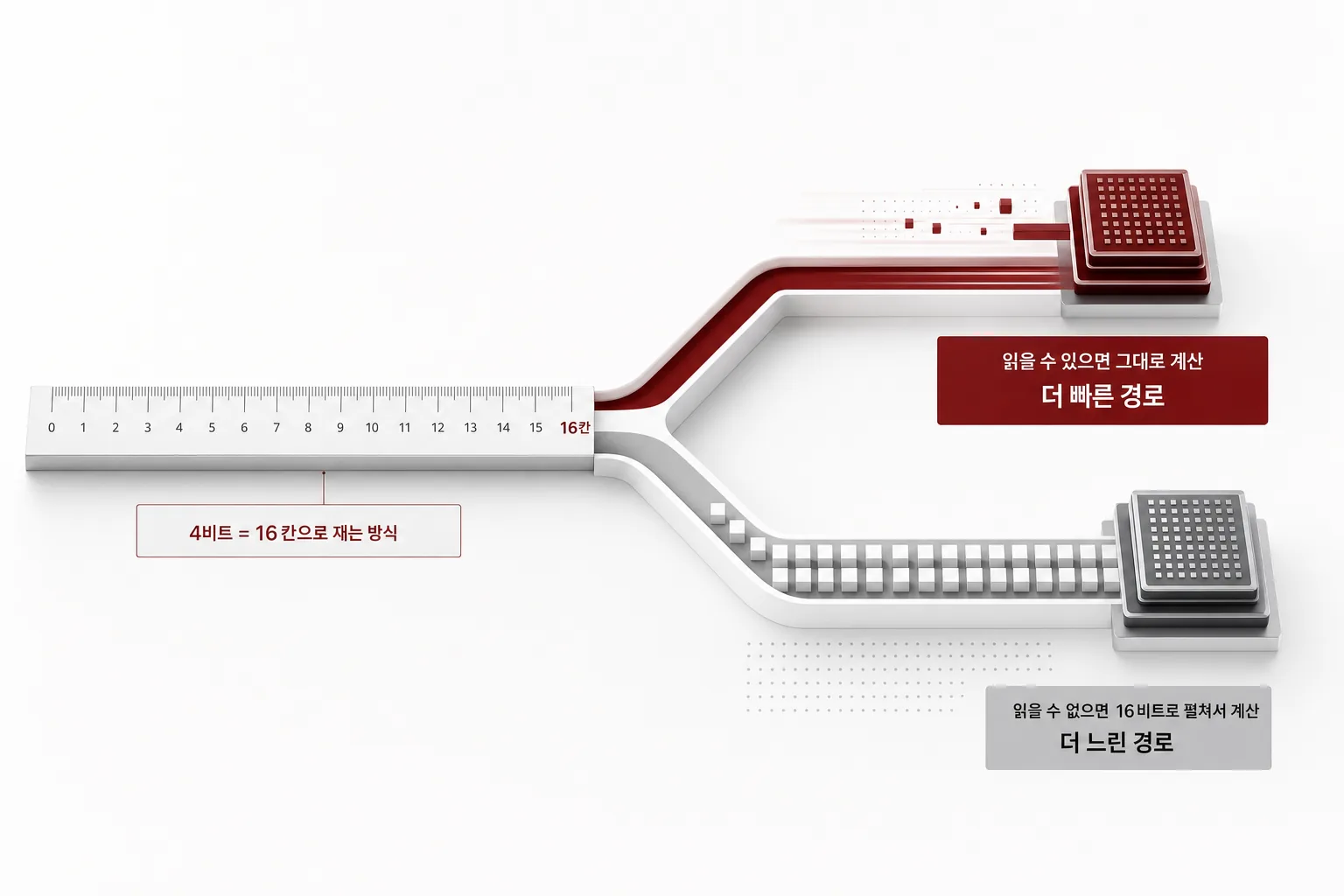 Four bits is a ruler with sixteen marks. Why that still produces usable results is the first half of this article.
Making the Heavy Books Thinner
In our earlier piece on speculative decoding we compared a large language model to a library. To write a single character the teacher has to haul several hundred very heavy books out of the stacks and spread them across the desk, and the actual reading takes an instant. Nearly all the time goes into moving the books.
Speculative decoding attacked how often you pull the books out. Quantization attacks the other side. It makes the books themselves thinner.
Thinner buys three things. More books fit in the stacks, so a model that did not fit on one GPU now does, and the leftover room takes more concurrent users. Moving them takes less time, so if a book is half as thick the trip is roughly half as long and characters come out faster. The third one is conditional. If you can read the book while it is still thin, the reading gets faster too. That third one is the one that most often fails to happen, and half of this article is about it.
A Ruler With Sixteen Marks
A model’s weights are, in the end, a few billion numbers. How finely you measure each one before writing it down is what quantization decides.
Sixteen bits gives you roughly sixty-five thousand marks to choose from. Eight bits gives you 256. Four bits gives you sixteen. Here is the complete set of values the four-bit floating point format E2M1 can represent.
0, 0.5, 1, 1.5, 2, 3, 4, 6 (and the negative of each)
That is the whole ruler. Eight positive values and eight negative ones. The first time you see it, the idea that a language model runs on this is hard to accept. With only that ruler, it does not.
So You Re-Fit the Ruler for Every Neighborhood
This is the heart of four-bit quantization, and it decodes half the labels on its own.
Suppose you have to measure people’s height with a ruler that has sixteen marks. Covering adults and newborns with the same ruler means the marks sit so far apart that nothing gets measured properly. But measuring a single third-grade classroom changes the problem. Those children are between 130 and 145 centimeters, so dividing just that range into sixteen gives you roughly centimeter resolution.
That is exactly the trick. Weights get grouped a few dozen at a time, and each group stores its own scale. Values inside a group are close to one another, so sixteen marks separate them well enough.
Two questions remain: how many values per group, and at what precision do you record the scale. The difference between NVFP4 and MXFP4 is precisely those two answers.
MXFP4 comes from the OCP microscaling standard. It groups 32 values and records the scale as E8M0, which has an exponent and no mantissa, so it expresses powers of two only. Two, four and eight are available; 1.5 is not. NVIDIA’s NVFP4 groups 16 values, a finer cut, and records the scale as FP8 E4M3, so awkward multipliers like 1.5x and 2.5x are on the table. It then layers an FP32 scale across the whole tensor on top. Fit a ruler per neighborhood, then fit one more for the whole city.
The price is size. Attaching an eight-bit scale to every sixteen values adds half a bit per value, so NVFP4 is called four bits and costs an effective 4.5. No precision is free.
Weights Are Easy, Today’s Ingredients Are Hard
There is one more layer to peel. Two kinds of numbers get multiplied inside a model.
Weights are fixed once training ends. They are like a recipe the cook has memorized, so you can study them at leisure and pick an optimal ruler in advance. Activations are recomputed every time depending on what the user typed. They are the ingredients that arrived this morning, and you cannot inspect them ahead of time.
Occasionally something unusually large arrives among those ingredients. These are called outliers, and a channel can come in around twenty times larger than its neighbors. The damage is that the scale stretches to cover that one big value and every ordinary value collapses into the same bucket. One three-meter-tall person in the classroom and every child’s height gets recorded as zero marks.
Hence the notation. W4A16 means weights down to four bits with activations left at sixteen. W8A8 puts both at eight, W4A4 puts both at four. Each step is harder than the last.
Methods for handling outliers followed. SmoothQuant applies a mathematically equivalent transform that pushes the difficulty out of the activations and into the weights, which can absorb it because you get to look at them in advance. QuaRot and SpinQuant go further and apply an output-preserving rotation that spreads the outliers evenly across many channels, trading one three-meter person for several slightly tall ones. That rotation is what brought W4A4, four bits on both sides, into practical range.
Measure Only What Matters, Finely
The other big idea is this. Not every layer matters equally.
Some layers can be crushed to four bits with almost no change in the output. Others start producing nonsense the moment you touch them. So the win goes to whoever keeps the important layers precise and cuts hard everywhere else. Most current methods are, in effect, competing over how to find out which layers those are.
llama.cpp’s importance matrix (imatrix) is the most direct answer. It runs representative text through the model, measures how much each weight influences the output, and feeds that into the quantizer. Formats with IQ in the name were designed assuming this matrix exists, and quality visibly collapses if you build them without one.
GPTQ quantizes one weight and then compensates for the resulting error by adjusting the remaining weights, using second-order information to solve “we lost this much rounding that value, so shift the neighbor to make it up.” AWQ looks at activation distributions instead, finds the top one percent of channels that fire large most often, and protects only those. It overfits its calibration set less, so it travels to other domains better. HQQ skips calibration data entirely and works from the weight distribution alone, quantizing a 70B model in five minutes.
Unsloth Dynamic pushes the idea to the file level. It assigns different bit widths per layer and recomputes that assignment per model. The UD- prefix on a filename is the marker. Dynamic 3.0, released in August 2026, says it widened its calibration sources to include agentic coding and multilingual conversation.
One warning in the Unsloth documentation deserves attention. Do not use the one-bit files for agents or tool calling. There is a cliff below two bits where accuracy falls away sharply, and that cliff shows up in call-a-tool-and-read-the-result work before it shows up in short question answering. If the smallest file looked appealing and your agent then started behaving strangely, this is usually why.
MLX on the Mac sits on the same trend. mlx_lm.dwq takes the original model as a teacher and distills only the parameters that do not get quantized, meaning the scales and biases. Rather than fitting the ruler by a fixed rule, it learns the marks, which cuts the loss at the same four bits. mlx_lm.dynamic_quant measures per-layer sensitivity and allocates bits automatically.
Do Not Trust the Label
This is where practitioners trip. Seeing Q4_K_M you naturally read “ah, four bits.” It is not.
We once opened a Qwen2.5-0.5B Q4_K_M file and counted it tensor by tensor. The genuinely four-bit Q4_K tensors accounted for 6.1 percent of the file, and the effective bit width of the whole file was not 4 but 6.16. The rest was eight-bit and six-bit tensors plus normalization parameters left at full 32. The label is closer to a recipe name than a bit count.
The same effect is visible in the repository that prompted this article. Unsloth’s GGUF build of Qwen3.8-Flash-Next offers seven UD variants, and the smallest one-bit file is 72.5GB while the largest four-bit file is 111GB. The bit counts differ fourfold and the sizes differ by 1.5x. The one-bit label does not mean every weight was crushed to one bit. It means “the most aggressive mix.”
So when picking a file, do not infer size from the number in the label. Read the file size that is printed. Whether that number fits your RAM is the question you actually need answered.
The Fork That Matters Most: Storage or Compute
Now the most important part. Miss this and the rest of the knowledge spins in place.
Storing weights in four bits does not mean the arithmetic happens in four bits. In most cases the GPU unpacks those four bits back to sixteen immediately before the multiply. That unpacking is itself computation, so it is not free.
Back to the library. You vacuum-sealed the books flat and shelved them. Hauling got easier. But to read one at the desk you have to unseal it back to full thickness every time. Carrying time went down and unsealing time appeared.
For that to be a net win, a condition has to hold. When hauling is the bottleneck, meaning few concurrent users and idle compute, you come out ahead. When users pile in and the GPU is already saturated with arithmetic, the unsealing lands on top of that saturated arithmetic and you lose.
Real four-bit compute is different. If the GPU contains circuitry that multiplies four-bit numbers while they are still compressed, no unpacking is needed. Hauling drops and arithmetic speeds up. That circuitry is the tensor core, and which generation ships tensor cores for which precision is the central table of this article.
The same four-bit file takes one of these two paths, and that decides the speed. The left path saves memory and loses time.
Telling the two apart is worth knowing. Look at which kernel your serving engine actually called. If it lands on a general matrix-multiply kernel like aten.mm.default, it is unpacking to compute. If an FP4-specific kernel name appears, it is multiplying compressed. We hold a rule that no FP4 speed number gets quoted without kernel-path evidence from the same run, because we fell into this trap repeatedly.
One more place to watch. Quantizing in PyTorch with NVIDIA’s Model Optimizer produces a simulation. NVIDIA’s own documentation states this directly: it only simulates the low-precision computation. It is for checking accuracy, and the actual speed and memory gains arrive only after export to TensorRT-LLM or vLLM. If you measured in PyTorch and wondered why four bits did not get faster, this is why.
So Which GPU Reads Which Ruler
Here is the table people find most confusing. Whether a precision can be stored and whether it can be multiplied are different questions, and this one is about multiplying.
| Hardware | FP8 tensor cores | FP4 tensor cores |
|---|---|---|
| RTX 4090, L40S (Ada) | yes | no |
| H100, H200 (Hopper) | yes | no |
| B200, GB200 (Blackwell datacenter) | yes | yes |
| RTX 50 series (Blackwell consumer) | yes | yes |
| AMD MI300X (CDNA3) | yes | no |
| AMD MI355X (CDNA4) | yes | yes (MXFP4) |
| Apple M1 through M4 | no | no |
| CPU | no | no |
The cell most often misread is H100 and H200. A large share of the GPU servers running today are that generation, and because they are excellent modern hardware it is easy to assume FP4 comes along for the ride. It does not. FP4 tensor cores start at Blackwell.
So what happens when you put a four-bit model on an H200? Memory savings are real. But every multiply unpacks first, so you pay the unsealing cost described above. It ends up slower than FP8.
Three Things That Surprised Us When We Measured
That last paragraph is not inference, it is measurement. We put Qwen3-Coder-30B-A3B on the same engine (vLLM 0.27.1) and changed only the GPU. The figures are medians across the concurrency 32 to 128 band.
The first surprise was that four bits lost. On H200, weight-only W4A16 came in at 0.81x to 0.84x of FP8. We built and served a four-bit file and it ran slower than eight-bit.
The second was stranger. Moving the same W4A16 to newer hardware, a B200, should help. It gets worse. The ratio falls from 0.76x to 0.67x. Thinking it through, this is inevitable. The faster the low-precision tensor cores get, the further behind a path that ignores them and unpacks instead falls. Using four bits wrongly costs more on newer silicon, not less.
On the same B200, running NVFP4 properly gives 1.22x to 1.28x over FP8. Same four-bit family, and W4A16 sits at 0.67x while NVFP4 sits at 1.28x. Nearly a factor of two decided by the kernel path, not the format name.
The third surprise was on quality. MXFP4 scored higher than NVFP4 on HumanEval (0.9268 versus 0.9024). But it ran at 0.66x to 0.74x of NVFP4’s speed. Both reached a native FP4 kernel on the B200, just not the same one: NVFP4 gets TensorRT-LLM’s fused MoE kernel and MXFP4 gets a CUTLASS path. Kernel maturity decided it, not the numeric format, which means this particular gap could invert later.
| On B200, versus FP8 (concurrency 32/64/128) | Throughput ratio | HumanEval |
|---|---|---|
| NVFP4 | 1.28 / 1.26 / 1.22 | 0.9024 |
| MXFP4 | 0.84 / 0.89 / 0.90 | 0.9268 |
| W4A16 (weight-only four bits) | 0.76 / 0.71 / 0.67 | 0.9268 |
And the real prize turned out to be power, not throughput. In a separate experiment we put bf16 and NVFP4 head to head at saturation. Throughput was effectively tied (23,415 versus 23,771 tok/s, a 1.5 percent gap) while power split at 500W versus 867W. Per token of energy that is 1.71x. For anyone renting GPUs, that number enters the cost model more directly than a throughput multiple does.
One honest addition. The largest throughput lever we found in the same period was not quantization. Fixing two serving settings moved single-stream throughput by 18.77x. torch.compile was off and the concurrent-request limit was pinned at a default of 32. While format debates argue over 1.2x and 1.3x, one setting moved eighteen. Check your baseline configuration before you touch quantization.
On a MacBook
The Mac is a different story entirely. GPU memory and system memory are the same pool, so a 128GB Mac can hold a 128GB model outright. A GPU server at the same price cannot come close, which is why Macs are strong for local experimentation.
The ceiling is bandwidth instead. Every character generated requires reading all the weights again, so how many gigabytes per second you can read very nearly sets how many characters per second you get. The M4 Pro does 273GB/s, the M4 Max does 410GB/s or 546GB/s depending on configuration, and the M3 Ultra does 819GB/s. Dropping to four bits means reading less, which is why quantization almost always wins on a Mac.
Formats split two ways. GGUF is the file format of the llama.cpp ecosystem, and Ollama and LM Studio both consume it. It runs on CPU and on Windows and Linux, so portability is unmatched. MLX is Apple’s own framework, Mac-only in exchange for being tuned to the Mac. Measured comparisons report MLX ahead by 1.4x to 1.6x on dense models during generation and up to 3x on MoE models. Prompt ingestion is a different matter, where llama.cpp can lead, so if your pattern is many short fresh conversations the gap narrows.
One thing changed in 2026. From the M5, each GPU core carries a dedicated matrix unit called a Neural Accelerator. Apple’s own measurements put time to first token at 3.33x to 4.06x versus the M4. Calibrate the expectation carefully though. Generation speed itself improved only 1.19x to 1.27x, and Apple’s document explains why: generation is bound by memory bandwidth rather than compute, and the M5’s bandwidth rose from the M4’s 120GB/s to 153GB/s, which is 28 percent. The gain matches the bandwidth gain almost exactly.
One clarification is worth making. Apple does not state that this unit accelerates block-scaled FP4 in hardware. It published measurements from running an MXFP4 model. Saying “Macs have FP4 tensor cores now” goes further than the evidence.
The practical recommendation is simple. For Mac-only use, MLX at four bits is the balance point. To squeeze more quality, build the four-bit with mlx_lm.dwq; with RAM to spare, go to six or eight bits. If you share files with other operating systems or need CPU execution, use GGUF. For sizing, four-bit puts a 7B around 4 to 5GB, a 30B around 20GB, and a 70B around 40 to 48GB.
On a Server
Serving many concurrent users adds one more criterion: small batch or large batch.
At small batch the GPU has compute to spare and only memory is straining, so moving fewer weight bytes is itself the win. Weight-only four-bit like AWQ or GPTQ works well here. As batch grows the GPU fills with arithmetic, the unpacking cost starts to hurt, and the right answer becomes a format that lowers both weights and activations. On Hopper that is FP8; on Blackwell it goes to NVFP4. NVIDIA’s own selection guide recommends W4A16 below batch 4 and W8A8 at 16 and above.
Tooling has settled reasonably. In the vLLM world, quantize with llm-compressor, export to the compressed-tensors format, and vLLM reads it directly. AWQ, GPTQ, bitsandbytes, AMD Quark and torchao are all supported too.
# Build an FP8 W8A8 checkpoint with llm-compressor (conceptual)
pip install llmcompressor
# apply QuantizationModifier(scheme="FP8_DYNAMIC") in the recipe, then run oneshot

# Serve with vLLM
vllm serve <path-to-quantized-model> \
  --max-num-seqs 256 \
  --max-model-len 32768
--max-num-seqs is spelled out deliberately. Half of that 18.77x incident was this value. Pinned at its default, no amount of incoming concurrency opens the ceiling.
After starting up, check the kernel name in the logs. If a four-bit model is loaded and a general matrix-multiply kernel is being called, you are saving memory and losing speed. Benchmarking in that state and concluding “four bits is not worth it” gets you the wrong answer.
Does Quality Actually Drop
Honestly: our benchmarks cannot see a difference, and that is not a reason to relax.
In the hardware comparison above, all five arms landed within four HumanEval problems of one another. The benchmark’s resolution is 0.61 percentage points per problem, and rerunning an identical configuration moves it about that much anyway. On Qwen3-30B-A3B our NVFP4 scored MMLU 0.7743 against bf16’s 0.7779, statistically indistinguishable.
The problem is that these benchmarks are short exchanges. A 2025 EMNLP study evaluated five quantization methods across several models and reported that eight-bit loses around 0.8 percent, effectively nothing, while four-bit lost up to 59 percent on long-context tasks, with the loss growing as context lengthened. A separate study of reasoning found a difficulty-proportional pattern: at W4A4, GSM8K lost nothing while AIME dropped 4.17 percent. Easy problems survive the crushing; hard ones start failing first.
Multilingual remains contested. One study finds automatic metrics look mild while human evaluation registers a much larger drop; another finds English-calibrated K-quants do not disproportionately harm other languages. That is unsettled, so we will not write it as settled.
Our position follows. Failing to find a loss is not the same as there being none. That is why the top priority for our next quarter of quantization work is not measuring a new format but standing up one control arm. If you cannot trust the ruler, everything measured with it wobbles. On your side, if you are going to run four bits, measure it yourself on your own workload, specifically on long context and hard reasoning.
The Order to Decide In
Compressed into a decision sequence, it is four steps.
First, settle where it runs. Mac means MLX or GGUF, anything involving CPU means GGUF, an NVIDIA server means checking that GPU’s generation. This alone eliminates half the candidate formats.
Second, pick a format with a native path on that hardware. Blackwell means NVFP4; Hopper and Ada mean FP8. If the batch is small and memory is tight, weight-only four-bit like AWQ or GPTQ enters the picture. Choosing four bits on Hopper means buying memory, not speed, and you should make that choice knowingly.
Third, confirm size from the file size. We saw above that Q4 does not mean four bits.
Walk down this instead of memorizing format names. There are only three forks.
Fourth, verify the kernel path and the quality before concluding anything. Read the kernel name from the logs, and measure with the longest context and hardest task in your actual workload.
Wrapping Up
Quantization in one sentence: rewrite the numbers with a coarser ruler, then re-fit the ruler per neighborhood so the coarseness does not show. That much is a decade-old idea, and today’s competition is over which neighborhood gets how fine a ruler. imatrix, GPTQ, AWQ, Unsloth Dynamic and MLX DWQ are all different answers to that one question.
In practice, though, what decides the outcome is not those answers but the fit with your hardware. The same four bits become 1.28x on a B200 and 0.81x on an H200. Memorizing format names pays less than carrying two questions: does my GPU have tensor cores for this precision, and is the engine actually calling that kernel.
The trend is worth noting. Early on every vendor shipped its own format; now things are converging on the OCP microscaling spec. AMD’s newest accelerator carries the same MXFP4 natively, and OpenAI shipped gpt-oss with MXFP4 weights outright. Apple has begun adding matrix units as well. In a few years “does this format work on this chip” should hurt less than it does today. Until then, and especially on the Hopper-generation hardware widely deployed right now, checking this table before you choose is worth several multiples.
A large part of what our inference product Metis does is making sure tenants never have to make this call themselves. Which format goes on which GPU generation, and which serving settings send the kernel down the right path, is repetitive work once it has been decided properly a single time. And the property described above, that four bits fails first on hard reasoning, matters especially for Paxis. An agent calls a tool, reads the result and judges again within a single request, and that judgment is exactly the kind of difficulty benchmarks are poor at catching. Lowering bits to save cost and having an agent quietly get worse is the hardest failure to notice.
Every measurement of ours cited here came from in-house B200 and H200 machines on the same engine, recorded with its conditions in our ledger. For the deeper per-format story, see The Same Four Bits Land on Opposite Sides of FP8 and There Was Almost No Q4 Inside Q4_K_M.