The Omni Model Doesn’t Get a Seat Next to the Video Model

This is for platform engineers and architects weighing whether to bring multimodal workloads onto in-house GPUs. By the end you’ll know that choosing between one omni model and a pipeline of specialist models strung together isn’t a matter of taste, it’s arithmetic about what fits on a single card, and you’ll have the numbers to run that arithmetic yourself.

Here’s the conclusion up front. Loading the video model and the audio specialists together on one NVIDIA H200 takes 72.37 GiB, 51.8% of the card. Loading the video model and the omni model together takes 130.29 GiB, 93.2% of the card, which leaves 9.5 GiB for everything generation needs at run time. Video generation alone reaches 3.57 GiB above its resident footprint, so that pairing does not realistically fit. What the omni model bought for that footprint was a 1.34 percentage point drop in transcription error.

Add stages and the problem stops being compute. It becomes a fight for space.

Same Card, Same Waveform, Two Approaches

Multimodal generation currently splits into two camps. One is the omni approach, where a single model takes in text, images, audio, and video and produces all of them back out. The other is the pipeline approach, where a specialist model handles each job and the outputs get stitched together. A benchmark leaderboard won’t settle which is better, because the two approaches have entirely different cost structures.

So we put both on the same card and gave them the same job. A speech synthesis model reads a Korean paragraph and produces a waveform, and a transcription specialist and an omni model each transcribe that waveform independently. We also added a 49.34 second recording of a real person speaking, which comes with a ground truth script so we could score both models’ transcripts against the same reference.

The models were Wan 2.2 T2V A14B for video, Qwen3-TTS 1.7B for speech synthesis, Qwen3-ASR 1.7B for transcription, and Qwen3-Omni-30B-A3B for the omni model. All four are Apache 2.0, so pulling the weights domestically and running them carries no licensing constraint. As covered in an earlier post, models with territorial restrictions were never candidates to begin with, and this lineup is the practical consequence of that earlier finding.

The environment was a single H200 NVL with 139.8 GiB of VRAM, torch 2.11.0, transformers 5.14.1, and diffusers 0.39.0. Every number in this post came out of that one combination. Every weight came from our internal registry.

Don’t Plan Capacity From a Probe

The first number we noticed wasn’t one we set out to measure.

Pulling the transcription model, 3.81 GiB across 9 files, ran at 540 MiB/s. The omni model, 65.69 GiB across 24 files, ran at 297 MiB/s. The video model, 117.53 GiB across 49 files, ran at 308 MiB/s. All three used 16 threads.

These numbers move between runs. Pulling the same omni model at a different moment gave 470 MiB/s. It’s a shared object store, so it varies. That makes it hard to claim a clean rule like “more files means slower,” and what’s solid is the range: real multi file pulls landed between roughly 260 and 550 MiB/s.

What matters sits above that. When we previously benchmarked pulling a single object, we got 916 MiB/s. Build a capacity plan on that and you’d underestimate real transfer time by two to three times. A probe answers whether an endpoint is reachable, not how long the job will take.

The Audio Layer: Omni Is 2.26x Slower and 17x Bigger

We gave both models the same job: transcribing the same 49.34 second Korean recording.

	Specialist (transcription)	Omni
Model	Qwen3-ASR 1.7B	Qwen3-Omni 30B-A3B
Resident VRAM	3.83 GiB	65.72 GiB
49.3s transcription	2.107s	4.755s
Real-time factor	23.4x	10.4x
Character error rate	7.59%	6.25%

The omni model is 2.26x slower on latency and holds 17.16x the resident memory. Add the speech synthesis model in and the two piece specialist stack comes to 7.8 GiB resident, which means the single omni model alone uses 8.43x what the entire audio layer uses. What that bought was a 1.34 percentage point improvement in character error rate.

We left cold load time out of the table on purpose. When we measured it, the ordering flipped depending on which model loaded first. In one run the transcription model took 1.45s and the omni model 9.23s. In another the transcription model took 89.63s and the omni model 19.39s. Whichever loads first absorbs CUDA context setup and a cold page cache. Load time is a property of the cache state at that moment, not of the model, so it can’t be used to choose between them.

The two models also failed differently. The specialist kept mishearing “Claude” as “cloud,” while the omni model got that proper noun right but rewrote “every turn” as “every token.” If the domain vocabulary in your workload actually matters, that difference can outweigh the raw error rate gap.

One honest caveat belongs here too. Much of what’s left in the error counts isn’t a recognition failure, it’s a numeral transcription convention. The reference script spells numbers out the way “ten times” and “five minutes” would read in English, and both models transcribed them as digits instead. So the 1.34 percentage point gap indicates a direction rather than settling the question. It’s a thin basis for justifying seventeen times the card. The gap itself, though, came out identical to the decimal across two independent runs.

How we scored is worth stating too. Both models wrap their answers in clutter. The specialist prepends fragments of its chat template, and the omni model echoes the instruction it was given before starting its answer. Strip that clutter from only one side and the ranking inverts completely. Leave the omni model’s instruction echo in and its error rate comes out at 14.29%, which says the specialist is twice as accurate, the exact opposite of the finding. So we stripped the same class of clutter from both sides on the same terms, and the table above is what came out. In a benchmark comparing two models, asymmetric preprocessing produces a bigger number than the models themselves do.

The Video Layer: One Stage Is 46 Percent of the Card

The video model took 185.31 seconds to load from disk into VRAM and held 64.57 GiB resident. Despite the A14B in its name, it actually carries two full experts, so what sits resident is roughly double a single expert’s size, plus the encoder and decoder on top.

We fixed generation at 480x832 resolution and 20 steps and varied only the frame count. A 2.06 second clip took 49.2 seconds, a 3.06 second clip took 79.6 seconds, and a 5.06 second clip took 152.3 seconds. Taking frame count from 33 to 81, a 2.5x increase, pushed generation time up 3.1x, which raises the cost per second of video from 23.9 seconds to 30.1 seconds. That’s attention scaling quadratically with frame count, so longer clips get proportionally more expensive. Generating three 5 second clips and stitching them together beats generating one 15 second clip in a single pass.

Reproducibility was solid. Repeating the same settings varied by under 0.09 seconds, and even the warmup run we planned to throw away landed almost identically to the real ones. Diffusion works through a fixed number of steps honestly every time, so there’s little room for it to wander. Unlike a language model, where generation time swings with token count, that makes capacity planning easier here, not harder.

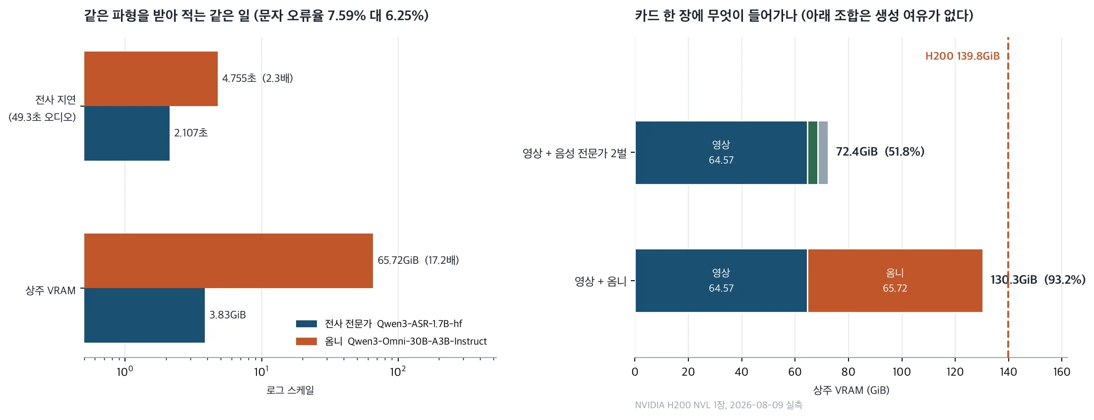On the left, latency and resident memory for the two approaches to transcribing the same waveform. On the right, what fills one card once you add the video stage. Both panels are measured on the same single H200.

So the Arithmetic Ends Like This

Now we can measure both options against the same yardstick.

Keeping the whole specialist pipeline resident adds the video model’s 64.57 GiB to the two audio specialists’ 7.8 GiB, for 72.37 GiB, 51.8% of the card. With more than half the card free, there’s room for active memory during generation and headroom left over. The cost of crossing a stage boundary drops to zero.

Swapping the omni model in for the audio layer adds the video model’s 64.57 GiB to the omni model’s 65.72 GiB, for 130.29 GiB, 93.2% of the card. That leaves 9.5 GiB, and video generation alone climbs 3.57 GiB above its resident footprint. It clears on paper with no operating room behind it.

This flips a common intuition. It’s tempting to assume folding everything into one model takes up less room, but in this combination it was the opposite. The audio specialists are small enough that the pipeline’s footprint is already down near rounding error territory. What actually eats the card isn’t the number of stages, it’s the single video model.

So the judgment comes down to this. In layers where the specialist models are small, like audio and language, the pipeline wins almost every time. For the omni model to win, its accuracy gain has to be large enough to justify ten plus times the resident footprint, and in this measurement it was 1.34 percentage points. The picture changes if the specialist model in each layer is roughly as large as the omni model itself. Then you’re paying a swap cost at every boundary, and reloading the exact same model took 195.28 seconds on its own, which adds more than three minutes in front of every request.

What Serving and Orchestration Need to Know

For an inference serving layer like Metis, the unit of scheduling has mostly been a single model. Multimodal workloads arrive as a bundle of stages instead, and whether that bundle fits together on one card changes response time by minutes, not milliseconds. What the scheduler needs to know isn’t the size of each individual model, it’s the resident footprint of the whole bundle. Placing the stages of one pipeline on the same card isn’t an optimization, it’s closer to a correctness requirement.

For a layer that executes multi model workflows, like Paxis, an ordering problem remains. Batch work that shares a stage together and swaps drop. Bounce between stages job by job and swaps climb. The throughput gap between a scheduler that knows the number 195 seconds and one that doesn’t is bigger than the gap you’d get from swapping in a better model.

Wrapping Up

Measured on the same card with the same waveform, the omni model cut transcription error by 1.34 percentage points at the cost of 2.26x the latency and 17x the resident memory. The two audio specialists together only cost 7.8 GiB, so the pipeline’s footprint is close to negligible, and what actually fills the card is the single video model. So if you’re serving video and speech together, the pipeline fits on one card and the omni model doesn’t.

The expectation that an omni model saves you resident slots only holds when every specialist in the stack is roughly as large as the omni model itself. In a layer like speech, where the specialists are small, that expectation flips.

Every number in this piece was measured directly on a single NVIDIA H200 NVL on August 9, 2026, and the omni model and the transcription specialist received the exact same waveform inside the same process. The measurement scripts and raw results are kept in our internal repository.